4K Aliasing
- Motivation: Optimising Memory Layout
- Multi-Matcher
- Dynamic Array Offsets Prevent Autovectorisation
- What is 4K Aliasing?
- Demonstrating 4K Aliasing
Motivation: Optimising Memory Layout
How do you improve the performance of the software you write? Consolidating data into contiguous regions of address space is a generally useful approach because most programs are bottlenecked on memory access. The consolidation has a positive impact on performance because processors fetch data in cache lines, for two reasons.
- A contiguous and aligned layout minimises the total number of cache lines required to store the program data.
- The likelihood that data for subsequent operations is already in a cache line is increased by a dense layout.
The benefits are kind of obvious, but it takes some work to profit from this when using the JVM because of the layout of the heap.
One way to think about Java objects laid out throughout the heap is to think of a sausage; amidst the innards and the breadcrumbs there is a bit of meat. Java objects have headers of implementation defined size, usually 12 or 16 bytes, and are aligned, by default, on 8 byte boundaries.
This means if you have an array of objects which wrap a long:
class WordMask {
  long word;
}
Even assuming compressed references, you end up with the composition of a typical sausage: 12 bytes for the header, eight bytes for the word, four bytes of alignment shadow. That’s 33% meat.
For more details about JVM object layout, read Aleksey Shipilëv’s objects inside out.
If you have a collection of these WordMask objects, this will impact application performance in the two ways mentioned before:
- Three times more memory needs to be addressed and fetched to process the entire collection than is strictly necessary.
- If a cache line is 64 bytes, eight
longs could fit, but only two entireWordMaskobjects.
The way around this - and there’s a lot written about it - is to transpose the object graph so that you don’t have collections of wrappers but a wrapper of an array:
class WordMasks {
  long[] words;
}
Assuming compressed references again, this means you have 12 bytes of header, four bytes of array length, the data, and then 0-7 bytes of shadow at the end. The relative space wasted quickly becomes negligible as the array grows. People really do this (though often off-heap) to improve performance.
Multi-Matcher
I have a toy project called multi matcher which, given some classification rules, allows the construction of a decision tree which, when queried, will give all the classifications which apply to an input object. To my horror, I occasionally hear from people who are using it, or trying to. I wrote about what it does and how it works in another post, but it’s not really important. Recently I decided to improve its performance by improving the layout of its data, and, predictably got better than 2x performance gains from consolidation.
How far can you take this approach before you start running in to other problems? Once you have consolidated all your data and increased the likelihood that it fits densely in cache, you probably want to exploit SIMD. What if the object you started off with contained an array rather than a single field:
class BitsetMask {
  long[] words;
}
Does it make sense to concatenate the arrays to improve data density?
The basic - and very simple - idea in multi-matcher is to assign an integer identity to each rule and decompose the set of rules by constraint. The evaluation starts off by assuming all rules apply by setting all the bits in a bit set. Then, values are extracted from the classified object and used to access the set of rules which accept the value. This set is intersected with the bit set. If the bit set becomes empty, the evaluation terminates. When there are no more values to extract, the bits left in the bit set are the rules which accept the input.
This reduces to doing something logically equivalent to the code snippet below:
    long[][] masks;
    public void match(long[] stillMatching, int id) {
      for (int i = 0; i < stillMatching.length; ++i) {
         stillMatching[i] &= masks[id][i];
      }
    }
Flattening the two-dimensional array is compelling for the sake of a dense layout.
    long[] masks;
    int size;
    public void match(long[] stillMatching, int id) {
      int offset = id * size;
      for (int i = 0; i < stillMatching.length; ++i) {
         stillMatching[i] &= masks[i + offset];
      }
    }
Do you think that this should make much difference beyond improving memory layout?
Dynamic Array Offsets Prevent Autovectorisation
C2 can autovectorise some code, such as the very simple loop above. The compiler does some analysis when it unrolls the loop, and notices blocks of the same instructions which don’t depend on each other except in the value of the induction variable. Some blocks of instructions can be replaced with special instructions which operate on vectors of several elements at once; it depends on the availability of a vector counterpart instruction. When this is successful, the code is much faster, and is especially effective when the input data is in cache. Vladimir Ivanov has slides on the topic.
I happened to know there was a limitation in C2’s autovectorisation when there are dynamic offsets into arrays. I knew this because I had encountered it investigating a weak matrix multiplication baseline and Vladimir actually explained in a comment what the problem was:
“Regarding C2 auto-vectorization issue, it’s a limitation in current implementation: compiler can’t prove different vectorized accesses won’t alias if index differs, so it gives up to preserve correctness (if aliasing happens, then different memory accesses can overlap and interfere which changes observable behavior).
The task in Java is simpler than in C/C++, but still it has to prove that source/destination arrays are different objects.
There’s a develop flag -XX:+SuperWordRTDepCheck (not available in product binaries, requires JVM recompilation), but it misses proper implementation (ptr comparisons) and just enables vectorization in such case.”
The comment did not survive migrating my blog to Github Pages, but I still have it in my email inbox and getting information like this directly from an expert like Vladimir is great.
What this means is that the code above can only be vectorised safely if the arrays certainly differ or if the vector width divides the offset. If there’s an offset, the compiler needs to prove that the arrays are different, and instead C2 just gives up rather than do the wrong thing.
I wrote a quick benchmark to convince myself that pursuing better locality by flattening a long[][] would be counter-productive.
The results are noisy because they were run on an otherwise busy laptop (Ubuntu 18, JDK11, Skylake mobile class CPU).
The point was to show that avoiding the offset would be much better; outside any reasonable measurement error, and I was more interested in checking the disassembly anyway.
Benchmark                  (offset)  (sourceSize)  (targetSize)   Mode  Cnt   Score   Error   Units
intersection                      0          1024           256  thrpt    5   6.118 ± 1.049  ops/us
intersection                    256          1024           256  thrpt    5   8.025 ± 1.413  ops/us
intersection                    512          1024           256  thrpt    5   6.099 ± 1.363  ops/us
intersection                    768          1024           256  thrpt    5   8.005 ± 1.472  ops/us
intersectionNoOffset              0          1024           256  thrpt    5  13.596 ± 1.724  ops/us
This difference is (partially - there’s more to this post) explained by autovectorisation when there is no offset. Here with no offset (reference).
  5.26%      │││  ↗││  0x00007f844c3f6aa0: vmovdqu 0x10(%r11,%rdx,8),%ymm0
  3.10%      │││  │││  0x00007f844c3f6aa7: vpand  0x10(%r8,%rdx,8),%ymm0,%ymm0
 12.08%      │││  │││  0x00007f844c3f6aae: vmovdqu %ymm0,0x10(%r8,%rdx,8)
  2.94%      │││  │││  0x00007f844c3f6ab5: vmovdqu 0x30(%r11,%rdx,8),%ymm0
  9.36%      │││  │││  0x00007f844c3f6abc: vpand  0x30(%r8,%rdx,8),%ymm0,%ymm0
 14.32%      │││  │││  0x00007f844c3f6ac3: vmovdqu %ymm0,0x30(%r8,%rdx,8)
  2.34%      │││  │││  0x00007f844c3f6aca: vmovdqu 0x50(%r11,%rdx,8),%ymm0
  2.00%      │││  │││  0x00007f844c3f6ad1: vpand  0x50(%r8,%rdx,8),%ymm0,%ymm0
 12.54%      │││  │││  0x00007f844c3f6ad8: vmovdqu %ymm0,0x50(%r8,%rdx,8)
  1.34%      │││  │││  0x00007f844c3f6adf: vmovdqu 0x70(%r11,%rdx,8),%ymm0
  0.24%      │││  │││  0x00007f844c3f6ae6: vpand  0x70(%r8,%rdx,8),%ymm0,%ymm0
 15.32%      │││  │││  0x00007f844c3f6aed: vmovdqu %ymm0,0x70(%r8,%rdx,8)
Here with a zero but dynamically defined offset (reference).
           ││││││  0x00007f5afc3f6699: mov    0x10(%rax,%r13,8),%r10
  0.50%    ││││││  0x00007f5afc3f669e: and    %r10,0x10(%r9,%rsi,8)
 16.95%    ││││││  0x00007f5afc3f66a3: mov    0x18(%rax,%r13,8),%r10
  1.01%    ││││││  0x00007f5afc3f66a8: and    %r10,0x18(%r9,%rsi,8)
 18.76%    ││││││  0x00007f5afc3f66ad: mov    0x20(%rax,%r13,8),%r10
  1.83%    ││││││  0x00007f5afc3f66b2: and    %r10,0x20(%r9,%rsi,8)
 19.30%    ││││││  0x00007f5afc3f66b7: mov    0x28(%rax,%r13,8),%r10
  1.63%    ││││││  0x00007f5afc3f66bc: and    %r10,0x28(%r9,%rsi,8)
The results above confirmed my beliefs adequately, but this is where it actually gets interesting. Look at the pattern in the throughput as a function of offset; high at 256 and 768; low at 0 and 512. Whilst these measurements are very poor quality, there’s more to the pattern than noise. This leads to an interesting benchmarking pitfall relating to precise data layouts called 4K aliasing.
What is 4K Aliasing?
The pattern above - and I present some better measurements below - is caused by something called 4K aliasing which only happens on Intel hardware. When the processor loads data from memory, the load comes through a queue called the load buffer; when it writes data back out to memory it goes through the store buffer. The buffers are basically independent. In principle, any ordering of load and store events could be possible, just as if you implemented a pair of unsynchronised queues in software without taking measures to ensure ordering guarantees are met. The kinds of ordering guarantees made by these buffers determine the architecture’s memory model.
On x86 processors (like mine), the store and load buffers are each FIFO (this is not true on ARM, for instance). Stores cannot be reordered with older loads, but loads may be reordered with older stores if the address is different. The ability to reorder some of the loads with older stores is good for program performance and makes basic sense; the pending store couldn’t possibly change the data being loaded as it’s going to a different address. This just allows data to be loaded without waiting for an unrelated store to complete, which could take several cycles. Disallowing reordering of loads and older stores to the same address means that if, for whatever reason, a write must store to memory rather than to a register, the program will slow down and bottleneck on storing to that memory address.
How is this enforced? Whenever there is a load, it must be checked whether there is a pending store to the same address. If there is one, it means that the load must be stale: an earlier instruction, according to program order, should have already modified the data at that address. It’s just an implementation detail that the write hasn’t completed yet. The load needs to wait until the right data can be read, and is reissued.
The way Intel processors do this is by querying the store buffer for a pending store to the load’s address. If there is a match, the load is reissued, but the match is determined by checking the lower 12 bits of the address! This means that whenever there is a recent store to an address at any offset $2^{12}$ bytes or 4KB away from one being loaded, then the pending store aliases with the load. So the load will be spuriously reissued, slowing the program down by a few cycles every time this happens.
Demonstrating 4K Aliasing
This all means that benchmarks like the one above, where data from one array is written to another, are at risk of producing wildly different numbers depending on the precise locations at which data resides in memory. The variation due to location dependent effects can actually be very high. To illustrate this point, I wrote a more complex benchmark which implicitly varies the addresses of the allocated arrays. I was also curious to know if autovectorisation would also be disabled if the offset were static final, so included benchmarks with constants to match the dynamic offsets.
The simplest way to do this is to allocate an array between the two arrays, though this limits the smallest possible offset to the size of the array header.
The array’s header and data will be allocated into a TLAB in between the two arrays.
Since Java objects are 8 byte aligned by default, it doesn’t make sense to measure offsets smaller than a long.
To make sure the arrays are not moved by garbage collection, I use EpsilonGC.
I use JOL to record the addresses of the arrays just so I can check that the arrays are at the relative offsets I think they are.
In the benchmark below, the 1024 element source will be allocated somewhere, it doesn’t matter where, and will take up 8KB ignoring its (irrelevant) header.
Then the padding array will be allocated, which will take up between 16 bytes and 2KB of space between the source and target array.
The target is always 2KB.
Since source is allocated before target, when there is a zero offset into source, there should be between an 8KB-10KB distance between the read and the write.
So 4K aliasing effects should be seen at the start of the range but not the end.
When the offset is 256, the difference is 6KB-8KB; 4K aliasing should show up at the end but not the start, and so on.
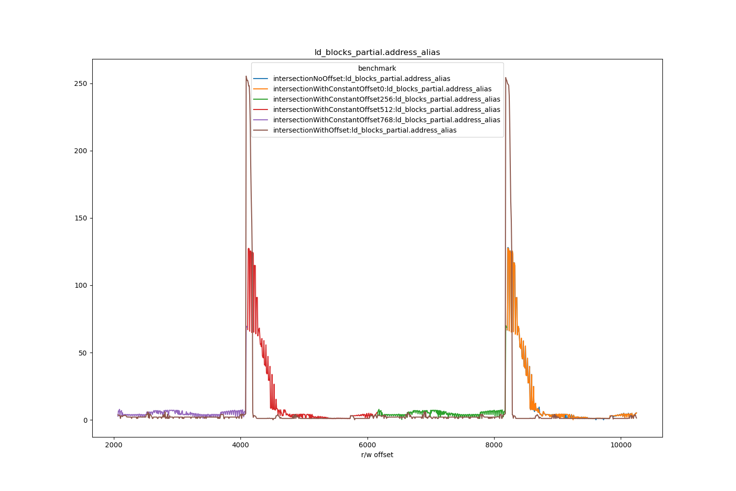
To prove 4K aliasing is happening, the counter ld_blocks_partial.address_alias can be tracked with -prof perfnorm.
public class LogicalAggregationBenchmark {


    public static void main(String... args) {
        for (int i = 0; i < 256; ++i) {
            System.out.println("\"" + i + "\", ");
        }
    }

    @State(Scope.Benchmark)
    public static class BaseState {

        long[] gap;

        @Param("256")
        int targetSize;

        @Param("1024")
        int sourceSize;

        @Param({"0","1","2","3","4","5","6","7","8","9","10","11","12","13","14","15",
                "16","17","18","19","20","21","22","23","24","25","26","27","28","29",
                "30","31","32","33","34","35","36","37","38","39","40","41","42","43",
                "44","45","46","47","48","49","50","51","52","53","54","55","56","57",
                "58","59","60","61","62","63","64","65","66","67","68","69","70","71",
                "72","73","74","75","76","77","78","79","80","81","82","83","84","85",
                "86","87","88","89","90","91","92","93","94","95","96","97","98","99",
                "100","101","102","103","104","105","106","107","108","109","110","111",
                "112","113","114","115","116","117","118","119","120","121","122","123",
                "124","125","126","127","128","129","130","131","132","133","134","135",
                "136","137","138","139","140","141","142","143","144","145","146","147",
                "148","149","150","151","152","153","154","155","156","157","158","159",
                "160","161","162","163","164","165","166","167","168","169","170","171",
                "172","173","174","175","176","177","178","179","180","181","182","183",
                "184","185","186","187","188","189","190","191","192","193","194","195",
                "196","197","198","199","200","201","202","203","204","205","206","207",
                "208","209","210","211","212","213","214","215","216","217","218","219",
                "220","221","222","223","224","225","226","227","228","229","230","231",
                "232","233","234","235","236","237","238","239","240","241","242","243",
                "244","245","246","247","248","249","250","251","252","253","254","255"})
        int padding;

        long[] source;
        long[] target;


        @Setup(Level.Trial)
        public void setup() {
            source = new long[sourceSize];
            gap = new long[padding];
            target = new long[targetSize];
            fill(source);
            fill(target);
        }

        private static void fill(long[] data) {
            for (int i = 0; i < data.length; ++i) {
                data[i] = ThreadLocalRandom.current().nextLong();
            }
        }
    }

    public static class ConstantOffset0State extends BaseState {
        private static final int offset = 0;
    }

    public static class ConstantOffset256State extends BaseState {
        private static final int offset = 256;
    }

    public static class ConstantOffset512State extends BaseState {
        private static final int offset = 512;
    }

    public static class ConstantOffset768State extends BaseState {
        private static final int offset = 768;
    }

    public static class DynamicOffsetState extends BaseState {
        @Param({"0","256","512","768"})
        int offset;
    }
}
As mentioned before the benchmarks themselves aim to exercise different behaviours.
- When the arrays are aggregated at the same index.
@Benchmark public void intersectionNoOffset(BaseState state, Blackhole bh) { var target = state.target; var source = state.source; for (int i = 0; i < state.target.length; ++i) { target[i] &= source[i]; } bh.consume(target); } - When the arrays are aggregated at static constant offsets of 0, 256, 512, 768.
@Benchmark public void intersectionWithConstantOffset0(BaseState state, Blackhole bh) { var target = state.target; var source = state.source; for (int i = 0; i < state.target.length; ++i) { target[i] &= source[ConstantOffset0State.offset + i]; } bh.consume(target); } - When the arrays are aggregated over a range of dynamic offsets which do not change once initialised.
 public static class DynamicOffsetState extends BaseState {
     @Param({"0", "256", "512", "768"})
     int offset;
 }

 @Benchmark
 public void intersectionWithOffset(DynamicOffsetState state, Blackhole bh) {
     var target = state.target;
     var source = state.source;
     int offset = state.offset;
     for (int i = 0; i < state.target.length; ++i) {
         target[i] &= source[offset + i];
     }
     bh.consume(target);
 }
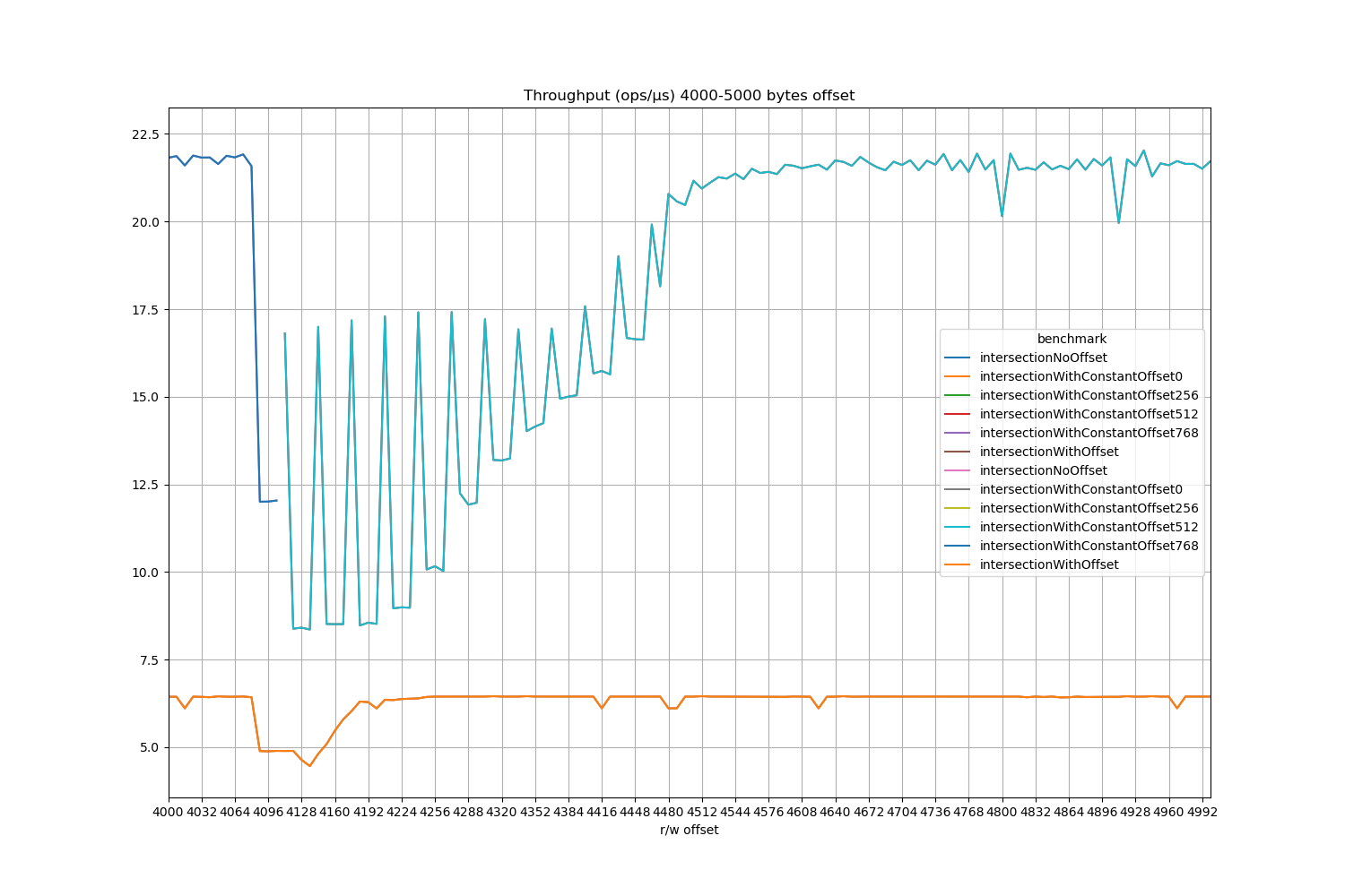
It turned out when the offsets are constant, the loop does get vectorised, and this gives an interesting comparison between scalar and vector code at and around the 4K offsets. 4K aliasing effects a much wider range of offsets when vector instructions are used than their scalar counterparts, and it depends on alignment too.
In these charts the total distance between an element in the source array and the target array is on the X axis.
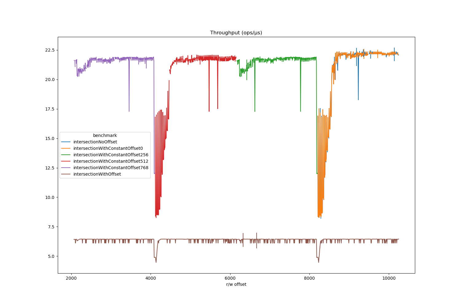
It also penalises vector code much more when loads are not 32-byte aligned (the oscillations just after the 4K dips have a period of 32 bytes).
What are the drops outside the vicinity of 4K offsets? I actually don’t know, probably an indication that I shouldn’t be benchmarking on a laptop.
The throughput aligns very well with ld_blocks_partial.address_alias.
The benchmark data is here.
The results have two interesting implications:
- Very similar code gets compiled completely differently according to seemingly tiny details like there being an offset or the offset being a compile time constant or not.
- Memory location - something you can’t even control - can have much larger effects than background noise.
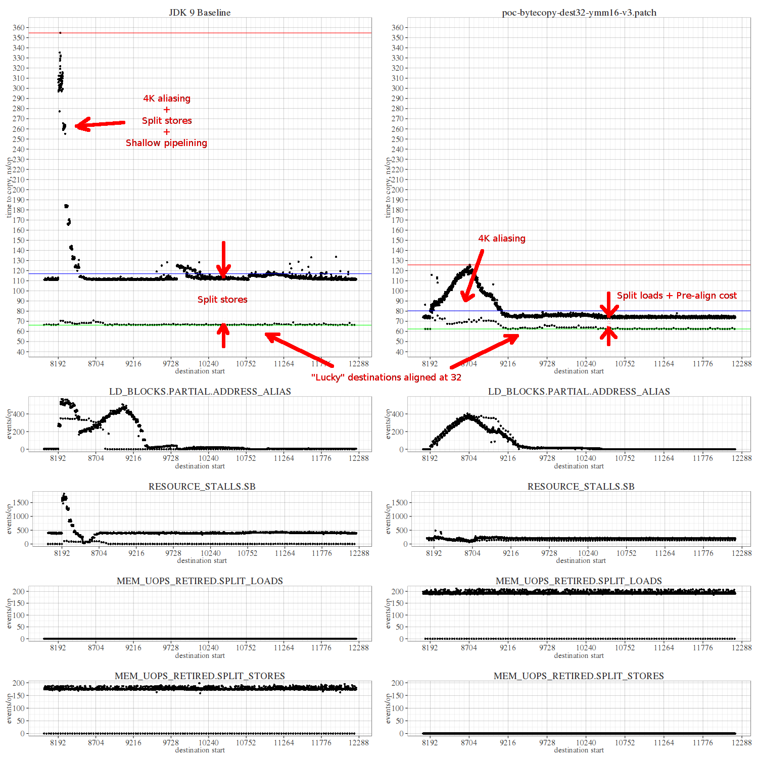
- Aleksey Shipilëv shared some revealing charts from his performance analysis of
System.arraycopy- particularly for AVX2. See JDK-8150730- I first came across 4K aliasing when I found similar patterns a few years ago. Vsevolod Tolstopyatov explained the cause of these patterns.