The Much Aligned Garbage Collector
A power of two is often a good choice for the size of an array. Sometimes you might see this being exploited to replace an integer division with a bitwise intersection. You can see why with a toy benchmark of a bloom filter, which deliberately folds in a representative cost of a hash function and array access to highlight the significance of the differential cost of the division mechanism to a method that does real work:
@State(Scope.Thread)
@OutputTimeUnit(TimeUnit.MICROSECONDS)
public class BloomFilter {

  private long[] bitset;

  @Param({"1000", "1024"})
  int size;


  @Setup(Level.Trial)
  public void init() {
    bitset = DataUtil.createLongArray(size);
  }

  @Benchmark
  public boolean containsAnd() {
    int hash = hash();
    int pos = hash & (size - 1);
    return (bitset[pos >>> 6] & (1L << pos)) != 0;
  }

  @Benchmark
  public boolean containsAbsMod() {
    int hash = hash();
    int pos = Math.abs(hash % size);
    return (bitset[pos >>> 6] & (1L << pos)) != 0;
  }

  private int hash() {
    return ThreadLocalRandom.current().nextInt(); // a stand in for a hash function;
  }
}
| Benchmark | Mode | Threads | Samples | Score | Score Error (99.9%) | Unit | Param: size |
|---|---|---|---|---|---|---|---|
| containsAbsMod | thrpt | 1 | 10 | 104.063744 | 4.068283 | ops/us | 1000 |
| containsAbsMod | thrpt | 1 | 10 | 103.849577 | 4.991040 | ops/us | 1024 |
| containsAnd | thrpt | 1 | 10 | 161.917397 | 3.807912 | ops/us | 1024 |
Disregarding the case which produces an incorrect result, you can do two thirds as many lookups again in the same period of time if you just use a 1024 element bloom filter. Note that the compiler clearly won’t magically transform cases like AbsMod 1024; you need to do this yourself. You can readily see this property exploited in any open source bit set, hash set, or bloom filter you care to look at. This is boring, at least, we often get this right by accident. What is quite interesting is a multiplicative decrease in throughput of DAXPY as a result of this same choice of lengths:
@OutputTimeUnit(TimeUnit.MICROSECONDS)
@State(Scope.Thread)
public class DAXPYAlignment {

  @Param({"250", "256", "1000", "1024"})
  int size;

  double s;
  double[] a;
  double[] b;

  @Setup(Level.Trial)
  public void init() {
    s = ThreadLocalRandom.current().nextDouble();
    a = createDoubleArray(size);
    b = createDoubleArray(size);
  }

  @Benchmark
  public void daxpy(Blackhole bh) {
    for (int i = 0; i < a.length; ++i) {
      a[i] += s * b[i];
    }
    bh.consume(a);
  }
}
| Benchmark | Mode | Threads | Samples | Score | Score Error (99.9%) | Unit | Param: size |
|---|---|---|---|---|---|---|---|
| daxpy | thrpt | 1 | 10 | 23.499857 | 0.891309 | ops/us | 250 |
| daxpy | thrpt | 1 | 10 | 22.425412 | 0.989512 | ops/us | 256 |
| daxpy | thrpt | 1 | 10 | 2.420674 | 0.098991 | ops/us | 1000 |
| daxpy | thrpt | 1 | 10 | 6.263005 | 0.175048 | ops/us | 1024 |
1000 and 1024 are somehow very different, yet 250 and 256 are almost equivalent. The placement of the second array, which, being allocated on the same thread, will be next to the first array in the TLAB (thread-local allocation buffer) happens to be very unlucky on Intel hardware for some array sizes. Let’s allocate an array in between the two we want to loop over, to vary the offsets between the two arrays:
  @Param({"0", "6", "12", "18", "24"})
  int offset;

  double s;
  double[] a;
  double[] b;
  double[] padding;

  @Setup(Level.Trial)
  public void init() {
    s = ThreadLocalRandom.current().nextDouble();
    a = createDoubleArray(size);
    padding = new double[offset];
    b = createDoubleArray(size);
  }
| Benchmark | Mode | Threads | Samples | Score | Score Error (99.9%) | Unit | Param: offset | Param: size |
|---|---|---|---|---|---|---|---|---|
| daxpy | thrpt | 1 | 10 | 2.224875 | 0.247778 | ops/us | 0 | 1000 |
| daxpy | thrpt | 1 | 10 | 6.159791 | 0.441525 | ops/us | 0 | 1024 |
| daxpy | thrpt | 1 | 10 | 2.350425 | 0.136992 | ops/us | 6 | 1000 |
| daxpy | thrpt | 1 | 10 | 6.047009 | 0.360723 | ops/us | 6 | 1024 |
| daxpy | thrpt | 1 | 10 | 3.332370 | 0.253739 | ops/us | 12 | 1000 |
| daxpy | thrpt | 1 | 10 | 6.506141 | 0.155733 | ops/us | 12 | 1024 |
| daxpy | thrpt | 1 | 10 | 6.621031 | 0.345151 | ops/us | 18 | 1000 |
| daxpy | thrpt | 1 | 10 | 6.827635 | 0.970527 | ops/us | 18 | 1024 |
| daxpy | thrpt | 1 | 10 | 7.456584 | 0.214229 | ops/us | 24 | 1000 |
| daxpy | thrpt | 1 | 10 | 7.451441 | 0.104871 | ops/us | 24 | 1024 |
The pattern is curious (pay attention to the offset parameter) - the ratio of the throughputs for each size ranging from 3x throughput degradation through to parity:
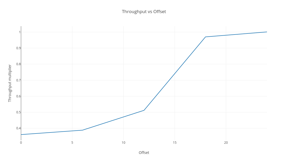
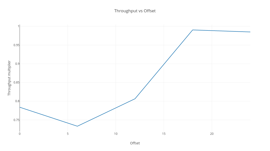
The loop in question is vectorised, which can be disabled by setting -XX:-UseSuperWord. Doing so is revealing, because the trend is still present but it is dampened to the extent it could be waved away as noise:
| Benchmark | Mode | Threads | Samples | Score | Score Error (99.9%) | Unit | Param: offset | Param: size |
|---|---|---|---|---|---|---|---|---|
| daxpy | thrpt | 1 | 10 | 1.416452 | 0.079905 | ops/us | 0 | 1000 |
| daxpy | thrpt | 1 | 10 | 1.806841 | 0.200231 | ops/us | 0 | 1024 |
| daxpy | thrpt | 1 | 10 | 1.408526 | 0.085147 | ops/us | 6 | 1000 |
| daxpy | thrpt | 1 | 10 | 1.921026 | 0.049655 | ops/us | 6 | 1024 |
| daxpy | thrpt | 1 | 10 | 1.459186 | 0.076427 | ops/us | 12 | 1000 |
| daxpy | thrpt | 1 | 10 | 1.809220 | 0.199885 | ops/us | 12 | 1024 |
| daxpy | thrpt | 1 | 10 | 1.824435 | 0.169680 | ops/us | 18 | 1000 |
| daxpy | thrpt | 1 | 10 | 1.842230 | 0.204414 | ops/us | 18 | 1024 |
| daxpy | thrpt | 1 | 10 | 1.934717 | 0.229822 | ops/us | 24 | 1000 |
| daxpy | thrpt | 1 | 10 | 1.964316 | 0.039893 | ops/us | 24 | 1024 |
The point is, you may not have cared about precise memory layout (not that you can really control it) much before because it’s unlikely you would have noticed unless you were really looking for it. Autovectorisation seems to raise the stakes enormously.
Analysis with Perfasm
It’s impossible to know for sure what the cause of this behaviour is without profiling. Since I observed this effect on my Windows development laptop, I use xperf via WinPerfAsmProfiler, which is part of JMH.
I did some instruction profiling. The same code is going to get generated in each case, with a preloop, main loop and post loop, but by looking at the sampled instruction frequency we can see what’s taking the most time in the vectorised main loop. From now on, superword parallelism is never disabled. The full output of this run can be seen at github. Here is the main loop for size=1024, offset=0, which is unrolled, spending most time loading and storing data (vmovdqu) but spending a decent amount of time in the multiplication:
  0.18%    0x0000020dddc5af90: vmovdqu ymm0,ymmword ptr [r10+r8*8+10h]
  9.27%    0x0000020dddc5af97: vmulpd  ymm0,ymm0,ymm2
  0.22%    0x0000020dddc5af9b: vaddpd  ymm0,ymm0,ymmword ptr [r11+r8*8+10h]
  7.48%    0x0000020dddc5afa2: vmovdqu ymmword ptr [r11+r8*8+10h],ymm0
 10.16%    0x0000020dddc5afa9: vmovdqu ymm0,ymmword ptr [r10+r8*8+30h]
  0.09%    0x0000020dddc5afb0: vmulpd  ymm0,ymm0,ymm2
  3.62%    0x0000020dddc5afb4: vaddpd  ymm0,ymm0,ymmword ptr [r11+r8*8+30h]
 10.60%    0x0000020dddc5afbb: vmovdqu ymmword ptr [r11+r8*8+30h],ymm0
  0.26%    0x0000020dddc5afc2: vmovdqu ymm0,ymmword ptr [r10+r8*8+50h]
  3.76%    0x0000020dddc5afc9: vmulpd  ymm0,ymm0,ymm2
  0.20%    0x0000020dddc5afcd: vaddpd  ymm0,ymm0,ymmword ptr [r11+r8*8+50h]
 13.23%    0x0000020dddc5afd4: vmovdqu ymmword ptr [r11+r8*8+50h],ymm0
  9.46%    0x0000020dddc5afdb: vmovdqu ymm0,ymmword ptr [r10+r8*8+70h]
  0.11%    0x0000020dddc5afe2: vmulpd  ymm0,ymm0,ymm2
  4.63%    0x0000020dddc5afe6: vaddpd  ymm0,ymm0,ymmword ptr [r11+r8*8+70h]
  9.78%    0x0000020dddc5afed: vmovdqu ymmword ptr [r11+r8*8+70h],ymm0
In the worst performer (size=1000, offset=0) a lot more time is spent on the loads, a much smaller fraction of observed instructions are involved with multiplication or addition. This indicates either a measurement bias (perhaps there’s some mechanism that makes a store/load easier to observe) or an increase in load/store cost.
  0.24%    0x000002d1a946f510: vmovdqu ymm0,ymmword ptr [r10+r8*8+10h]
  3.61%    0x000002d1a946f517: vmulpd  ymm0,ymm0,ymm2
  4.63%    0x000002d1a946f51b: vaddpd  ymm0,ymm0,ymmword ptr [r11+r8*8+10h]
  9.73%    0x000002d1a946f522: vmovdqu ymmword ptr [r11+r8*8+10h],ymm0
  4.34%    0x000002d1a946f529: vmovdqu ymm0,ymmword ptr [r10+r8*8+30h]
  2.13%    0x000002d1a946f530: vmulpd  ymm0,ymm0,ymm2
  7.77%    0x000002d1a946f534: vaddpd  ymm0,ymm0,ymmword ptr [r11+r8*8+30h]
 13.46%    0x000002d1a946f53b: vmovdqu ymmword ptr [r11+r8*8+30h],ymm0
  3.37%    0x000002d1a946f542: vmovdqu ymm0,ymmword ptr [r10+r8*8+50h]
  0.47%    0x000002d1a946f549: vmulpd  ymm0,ymm0,ymm2
  1.47%    0x000002d1a946f54d: vaddpd  ymm0,ymm0,ymmword ptr [r11+r8*8+50h]
 13.00%    0x000002d1a946f554: vmovdqu ymmword ptr [r11+r8*8+50h],ymm0
  4.24%    0x000002d1a946f55b: vmovdqu ymm0,ymmword ptr [r10+r8*8+70h]
  2.40%    0x000002d1a946f562: vmulpd  ymm0,ymm0,ymm2
  8.92%    0x000002d1a946f566: vaddpd  ymm0,ymm0,ymmword ptr [r11+r8*8+70h]
 14.10%    0x000002d1a946f56d: vmovdqu ymmword ptr [r11+r8*8+70h],ymm0
This trend can be seen to generally improve as 1024 is approached from below, and do bear in mind that this is a noisy measure. Interpret the numbers below as probabilities: were you to stop the execution of daxpy at random, at offset zero, you would have a 94% chance of finding yourself within the main vectorised loop. You would have a 50% chance of observing a load, and only 31% chance of observing a multiply or add. As we get further from 1024, the stores dominate the main loop, and the main loop comes to dominate the method. Again, this is approximate. When the arrays aren’t well aligned, we spend less time storing, less time multiplying and adding, and much more time loading.
| classification | offset = 0 | offset = 6 | offset = 12 | offset = 18 | offset = 24 |
|---|---|---|---|---|---|
| add | 22.79 | 21.46 | 15.41 | 7.77 | 8.03 |
| store | 12.19 | 11.95 | 15.55 | 21.9 | 21.19 |
| multiply | 8.61 | 7.7 | 9.54 | 13.15 | 8.33 |
| load | 50.29 | 51.3 | 49.16 | 42.34 | 44.56 |
| main loop | 93.88 | 92.41 | 89.66 | 85.16 | 82.11 |
The underlying cause is 4k aliasing which refers to the reissuing of loads which alias recent stores to the same address. For the sake of performance, loads and stores are allowed to race, which is innocuous if they are independent, but violations of memory ordering are checked for and repaired if necessary. To avoid write-after-read hazards, loads are reissued whenever there is a pending store to the same address in the store buffer, which costs a few cycles. On Intel CPUs, this is detected by inspecting the lower 12 bits of the load and store addresses, which means that these checks have false positives. Whenever an address at a 4K offset from a recently written value is loaded, the lower 12 bits match, and the load is reissued needlessly. That’s exactly what happens in DAXPY with these particular array sizes when they are contrived to sit next to eachother in a TLAB (1024 * 8 = 8K), with each array acccessed sequentially at a fixed offset. The 250 and 256 element arrays are at a 2K offset, so the addresses differ in the lower 12 bits.
The effect observed here is also a contributing factor to fluctuations in throughput observed in JDK-8150730.
Garbage Collection
Should you try to control the placement of your arrays to control quirks like this? In this microbenchmark, it’s easy to arrange that. Fortunately, this shouldn’t be necessary. True to the title, this post has something to do with garbage collection. The arrays were allocated in order, and no garbage would be produced during the benchmarks, so the second array will be allocated in the TLAB, at a controllable and fixed offset from the first array.
Let’s put some code into the initialisation of the benchmark bound to trigger garbage collection:
  String acc = "";

  @Setup(Level.Trial)
  public void init() {
    s = ThreadLocalRandom.current().nextDouble();
    a = createDoubleArray(size);
    b = createDoubleArray(size);
    // don't do this in production
    for (int i = 0; i < 10000; ++i) {
      acc += UUID.randomUUID().toString();
    }
  }
A miracle occurs: the code speeds up!
| Benchmark | Mode | Threads | Samples | Score | Score Error (99.9%) | Unit | Param: size |
|---|---|---|---|---|---|---|---|
| daxpy | thrpt | 1 | 10 | 6.854161 | 0.261247 | ops/us | 1000 |
| daxpy | thrpt | 1 | 10 | 6.328602 | 0.163391 | ops/us | 1024 |
Why? G1 has rearranged the heap and that second array is no longer right next to the first array, and the bad luck of the initial placement has been undone. This makes the cost of garbage collection difficult to quantify, because if it takes resources with one hand it gives them back with another.
The benchmark code is available at github.