Reservoir Sampling
Feedback on these posts is welcome and solicited. If you find mistakes, corrections can be made by pull request at GitHub.
In my last post I covered a technique to infer distribution parameters from a sample taken from a system with the aim of calibrating a simulation. This post is about how to take samples, using reservoir sampling algorithms.
This is not a subject I have ever had much exposure to; I have always trusted that libraries like Dropwizard Metrics just do the right thing. This ignorance is quite terrifying if you want to do something deeper than feed InfluxDB with numbers to populate Grafana dashboards. It’s important to understand how the numbers are generated. I decided to dig in to what was groundbreaking research in the 1980s to get a better understanding of how the algorithms work (it’s a fairly stable field…). I discovered that algorithms more efficient than the ones typically used were known about decades ago, but that it only really matters when measuring very low latency operations. There is an experimental evaluation at the end of the post.
This post is based on the notes I wrote reading these papers; the motivation for writing it was to focus my reading. Wherever the mathematical derivations in the papers are missing important steps or background which aid understanding, the derivations are reproduced with more detail here. The complete and easy to follow derivations have not been copied and are best read in situ.
A lot of the mathematical sections can be skipped.
- Background: Faster Methods for Random Sampling
- Reservoir Algorithms: Random Sampling with a Reservoir
- Implementations and Evaluation of Algorithms R, X, and Z
- References
- Further Reading
Background: Faster Methods for Random Sampling
It’s worth taking a look at the derivations of Algorithm A and Algorithm D in Vitter’s paper on Faster Methods for Random Sampling first. The algorithms were motivated by files stored on tape, and assumes that the number of records in the file is known prior to taking the sample. Tape storage, now antiquated, was a good motivator for streaming algorithms because going backwards was prohibitively slow. Both algorithms work by generating the number of records to skip, rather than performing a trial per record, which means the number of random numbers generated scales with the size of the sample rather than the input. Both draw these skips from the same distribution, but the algorithms differ in the way they transform uniform random variables to appropriately distributed random skips. Algorithm A employs linear search, making its complexity linear in the input, whereas Algorithm D inverts a distribution function and rejection-samples the results, making its complexity linear in the sample with higher constant factors.
Skipping Records
Though not about reservoir sampling, the paper is informative because it shows how to derive an approximately uniform distribution whilst streaming the input. Whilst the paper glosses over the details of the derivation, I found it instructive to reproduce the results by trundling through the combinatorics so you may find much of this section tedious. If you don’t read this section, the important outcome is that the distribution is approximately uniform without random access, so produces unbiased samples.
Suppose we want to select a sample of size $k$ from a large file of known size $m$ records. Vitter starts by defining the random variable $S(n, N)$ as the number of observations to skip, where $n$ is the number of records remaining to be selected, and $N$ is the number of records remaining in the file. In general, the sampling algorithm will
- Generate $s = S(n, N)$
- Skip over $s$ records
- Include the record at offset $s+1$ relative to the start of the scan in the sample.
We just need to be sure we define $S(n, N)~\in~[0, N-n]$ such that we do get $k$ samples by the time the input has been scanned, without introducing bias. It is intuitive that the probability of skipping $s$ records should be:
\[\mathbb{P}(S=s) = \frac{n}{N-s}\]Intuitively, when the size of the sample taken is small ($n \ll k$) we will skip fewer records; when there are many records left in the file ($N - s \sim 0$) we are more likely to take the next record. We need to skip on average $N/n$ records to get $n$ uniform samples, this is verified by deriving the density function and its moments.
The cumulative distribution function can be derived by setting up a recurrence relation:
\[\begin{aligned}F(s) &= \mathbb{P}(S \leq s) \\ &= 1 - \mathbb{P}(S > s) \\ &= 1 - \mathbb{P}(S > s - 1)\mathbb{P}(S = s)' \\ &= 1 - \mathbb{P}(S > s - 1)(1 - \frac{n}{N-s}) \\ &= 1 - (1 - F(s-1))(1 - \frac{n}{N-s}) \end{aligned}\]Defining $F(x) = 0$ whenever $x < 0$ we get:
\[\begin{aligned}F(0) &= \frac{n}{N}\\ F(1) &= 1 - (1 - \frac{n}{N})(1 - \frac{n}{N-1})\\ F(2) &= 1 - (1 - \frac{n}{N})(1 - \frac{n}{N-1})(1 - \frac{n}{N-2}) \\ &... \\ F(s) &= 1 - (1 - \frac{n}{N})(1 - \frac{n}{N-1})...(1 - \frac{n}{N-s}) \\ &= 1 - \prod_{i=0}^s(1 - \frac{n}{N-i}) \\ &= 1 - \prod_{i=0}^s(\frac{N-i-n}{N-i}) \\ &= 1 - \frac{(N-n)^\underline{s+1}}{N^\underline{s+1}} \end{aligned}\]The last step is made by inspection that the expression is a falling factorial.
Since $\mathbb{P}(S=s) = F(s) - F(s-1)$, the distribution function can be used to find the probability density function.
\[\begin{aligned}f(s) &= (1-\frac{(N-n)^\underline{s+1}}{N^\underline{s+1}}) - (1- \frac{(N-n)^\underline{s}}{N^\underline{s}})\\ &= \frac{(N-n)^\underline{s}}{N^\underline{s}} - \frac{(N-n)^\underline{s+1}}{N^\underline{s+1}}\\ &= \frac{(N-n)!}{(N-n-s)!}\frac{(N-s)!}{N!} - \frac{(N-n)!}{(N-n-s-1)!}\frac{(N-s-1)!}{N!}\\ &= \frac{(N-n)!(N-s)(N-s-1)!}{(N-n-s)(N-n-s-1)!N!} - \frac{(N-n)!(N-s-1)!}{(N-n-s-1)!N!}\\ &= \frac{((N-s) - (N-n-s))(N-n)!(N-s-1)!}{(N-n-s)(N-n-s-1)!N!}\\ &= \frac{n}{N}\frac{(N-s-1)!}{(N-1)!}\frac{(N-n)!}{(N-n-s)!}\\ &= \frac{n}{N}\frac{(N-n)^\underline{s}}{(N-1)^\underline{s}} \end{aligned}\]To get an unbiased sample, the mean and standard deviation need to be close to $N/n$.
Some standard properties of falling factorials can be used to convert this expression into one of binomial coefficients:
\[\begin{aligned} {N \choose n} &= \frac{N^\underline{n}}{n!} = \frac{N!}{n!(N-n)!}\\ {N-s-1 \choose n-1} &= \frac{(N-s-1)^\underline{n-1}}{(n-1)!} = \frac{(N-s-1)!}{(n-1)!(N-s-n)!}\end{aligned}\]These results can be plugged in to the density function to express it in terms of binomial coefficients.
\[\begin{aligned} f(s) &= \frac{n}{N}\frac{(N-n)^\underline{s}}{(N-1)^\underline{s}} \\ &= \frac{n}{N}\frac{(N-s-1)!}{(N-s-n)!}\frac{(N-n)!}{(N-1)!}\\ &= n(n-1)!{N-s-1 \choose n-1} \frac{(N-n)!}{N!} \\ &= \frac{N-s-1 \choose n-1}{N \choose n} \end{aligned}\]To calculate the first moment we need to derive two facts about sums of binomial coefficients.
\[\begin{aligned}\sum_{k=0}^{p} {k \choose m} &= {p+1 \choose m+1}(1) \\ \sum_{k=0}^{p} k {k \choose m}&=\sum_{k=0}^{p} (k+1-1) {k \choose m}\\ &= \sum_{k=0}^{p}\left((k+1) \frac{k!}{m! (k-m)!}-{k \choose m}\right)\\ &=\sum_{k=0}^{p}\left((k+1) \frac{k!}{m! (k-m)!}-{k \choose m}\right)\\ &= \sum_{k=0}^{p}\left((m+1) {k+1 \choose m+1}-{k \choose m}\right)\\ (1) \implies \sum_{k=0}^{p} k {k \choose m}&= (m+1) {p+2 \choose m+2}-{p+1 \choose m+1}(2) \end{aligned}\]Using equations (1) and (2) we can calculate the first moment and find it is close to $N/n$ as desired:
\[\begin{aligned} \mathbb{E}(S) &= \sum_{s=0}^{N-n}sf(s) \\ &= \frac{\sum_{s=0}^{N-n} s {N-s-1 \choose n-1}}{N \choose n}\\ &= \frac{\sum_{k=n-1}^{N-1} (N-k-1) {k \choose n-1}}{N \choose n} \end{aligned}\]Where $k=N-s-1$
\[\begin{aligned} &=\frac{\sum_{k=n-1}^{N-1} (N-1) {k \choose n-1}-\sum_{k=n-1}^{N-1} k {k \choose n-1}}{N \choose n}\\ (1), (2) \implies &= \frac{(N-1){N \choose n}-n {N+1 \choose n+1} + {N \choose n}}{N \choose n}\\ &= \frac{1}{N \choose n} \left( N {N \choose n}-n {N \choose n}\frac{N+1}{n+1} \right)\\ &= N - n\frac{N+1}{n+1}\\ &= \frac{N(n+1) -n(N + 1))}{n+1} \\ &= \frac{N - n}{n+1} \simeq \frac{N}{n}\\ \end{aligned}\]Similarly, the variance is close to $N^2/n^2$, and therefore the standard deviation is close to $N/n$.
\[\begin{aligned} Var(S) &= \sum^{N-n}s^2f(s) - \mathbb{E}(S)^2 \\ &= \frac{(N + 1)(N - n)n}{(n+2)(n+1)^2} \simeq \frac{N^2}{n^2} \end{aligned}\]So the probability density function is suitable.
Algorithm A
Algorithm A generates a uniform random variable $x \sim Unif(0,1)$ and searches for the smallest value of the next skip $s$ such that $x \leq F(s)$.
- Generate a random number $x \in [0, 1]$.
- Process the stream until position $s$ satisfies $(N-n)^\underline{s+1} \leq x N^\underline{s+1}$.
- Select the next record. Subtract $s+1$ from $N$ and decrement $n$.
The complexity of the algorithm is linear in the size of the file, but independent of the size of the sample. The algorithm generates $n$ random variables for a sample of size $n$. Algorithm B replaces linear search with Newton’s method.
Algorithm D
Algorithm D is the main contribution from Faster Methods for Random Sampling and builds on the analysis required for Algorithm A. Whilst many other derivations in this post are fleshed out in full, the derivations in this section of the paper are well presented and complete: there is little to gain from copying them here, so this section is less mathematical. Its distinguishing feature is that its complexity is independent of the number of records in the file; this is achieved by generating the skips using von Neumann rejection sampling. However, there is a high constant factor and this is only faster than Algorithm A if $n \ll N$, so the first thing the algorithm does is test the ratio $n/N$ against a threshold and will fall back to Algorithm A if the threshold is breached.
The skips are modeled by a random variable $X$ with probability density function $g(x)$, which must satisfy the condition
\[f(x) \le cg(x)\]For some constant $c$. For the acceptance test, we also need a uniform random variable $U$, generating $u \sim U$ and $G^{-1}(x)$, verifying that $ u \ge f(x)/cg(x) $, otherwise trying again.
The explanation of rejection sampling on Wikipedia is brilliant, so I included it here for context.
“To visualize the motivation behind rejection sampling, imagine graphing the density function of a random variable onto a large rectangular board and throwing darts at it. Assume that the darts are uniformly distributed around the board. Now remove all of the darts that are outside the area under the curve. The remaining darts will be distributed uniformly within the area under the curve, and the x-positions of these darts will be distributed according to the random variable’s density. This is because there is the most room for the darts to land where the curve is highest and thus the probability density is greatest.” Source: Wikipedia
As a performance optimisation, if there is a function $h(x) : h(x) \le f(x) \forall x$, it can substitute $f(s) = f(\lfloor x \rfloor)$, and $f(s)$ only need be evaluated when $u \ge h(x)/xg(x)$. The algorithm is specified as follows:
- If $ n \ge aN$ for some constant $a$, use Algorithm A.
- Consume the input: for each $i~\in~[0, n)$ generate $s_i$ by rejection sampling, keep trying until successful.
- Skip $s_i$ records, and keep the next record (i.e. the one at relative offset $s_i+1$).
The faster the generation phase, the better: there is a tradeoff between the cost of evaluating the inverse of the distribution function and rate of rejection. Given enough time, any distribution could generate a point which could have been drawn from $F(s)$, so long as the distribution’s range covers $[0, N)$. The best distribution to use is the one closest to $F(s)$. Vitter presents two different distribution functions which can approximate $F(s)$, depending on the value of $n^2/N$.
Skip generation when $n^2$ small relative to N
When $n^2/N$ is small, the beta distribution is used, with $\alpha=0, \beta=n$.
\[g(x) = \frac{n}{N}\left( 1-\frac{x}{N} \right)^{n-1}\]To use it, we need to transform uniform random variables into beta distributed random variables, so need the distribution function and its inverse.
\[\begin{aligned} G(x) &= \mathbb{P}(X \le x)\\ &= 1 - \left(1 - \frac{x}{N} \right)^n\\ \implies G^{-1}(y) &= N(1 - (1-y)^{1/n}) \end{aligned}\]These are standard results of the beta distribution. If $y$ is drawn from a uniform distribution, then so is $1-y$, which saves a subtraction, and allows $X$ as:
\[x = N(1 - e^{y/n})\]With $s$, when $x$ is accepted, defined as $s= \lfloor x \rfloor$. The constant is given by:
\[c = \frac{N}{N-n+1}\]The function $h(s)$ is given by
\[h(s) = \frac{n}{N}\left( 1 - \frac{s}{N-n+1} \right)^{n-1}\]Detailed proof of the suitability of these choices is given in the paper, and there is no clarity to be added by reproducing them here.
Skip generation when $n^2$ large relative to N
When $n^2/N$ is large, the geometric distribution is used.
\[g(s) = \frac{n-1}{N-1}\left(1 - \frac{n-1}{N-1}\right)^s\]We have the well known inverse distribution function:
\(s = \Bigl\lfloor \frac{-y}{\ln \left(1 - \frac{n-1}{N-1} \right)} \Bigr\rfloor\).
The constant is given by
\[c = \frac{n}{n-1}\frac{N}{N-1}\]The function $h(s)$ is given by
\[h(s) = \frac{n}{N}\left( 1 - \frac{n-1}{N-s} \right)^s\]Again, a readable proof of the suitability of these choices is given in the paper.
The remainder of the coverage of the algorithm considers computational optimisations which are unlikely to be relevant in 2020.
Reservoir Algorithms: Random Sampling with a Reservoir
Knowing the number of records in the file is quite a limitation if we want to draw samples from an application which runs for arbitrary periods of time. Reservoir sampling solves this problem by keeping a reservoir of sampled data which is maintained (added to and evicted from) so that it is always an unbiased sample of the data seen so far. The elements of the reservoir are replaced with some probability chosen to maintain the quality of the sample. This section includes three algorithms: R, X, and Z, written about in Random Sampling with a Reservoir. Algorithm R is a computationally inefficient, but widely used, algorithm which generates as many random variables as there are inputs. Algorithms X and Z are analogous to A and D: they both generate numbers of records to skip; X performs linear search; Z rejection samples the inverse of an approximation to the skip distribution.
Algorithm R
Algorithm R predates Vitter’s work on Algorithm A. It is presented on page 144 of The Art of Computer Programming Volume 2 and is credited to Alan Waterman, but is also covered in Random Sampling with a Reservoir. The algorithm works as follows:
- Initialise the reservoir with capacity $k$
- Store the first $k$ values seen.
- When the reservoir is full, for each record generate a random variable $x~\in~[0, t)$ where $t$ is the position of the record in the stream.
- If $x < k$ replace the record at position $x$ of the reservoir, otherwise discard it.
Note that a random number is generated for each record in the input. Incidentally, this is the algorithm used by Dropwizard metrics, where it is incorrectly attributed to Vitter, and seems not to recognise Algorithm R’s purported inferiority to the algorithms introduced by the paper.
/**
 * A random sampling reservoir of a stream of {@code long}s. Uses Vitter's Algorithm R to produce a
 * statistically representative sample.
 *
 * @see <a href="http://www.cs.umd.edu/~samir/498/vitter.pdf">Random Sampling with a Reservoir</a>
 */
public class UniformReservoir implements Reservoir {
Does Algorithm R produce uniformly distributed samples?
Whilst Vitter’s derivations are all constructive (i.e. they produce concrete distribution and density functions, and their moments) it’s a lot easier to reason about uniformity inductively.
First, note that until there are $k$ items in the reservoir, no replacement takes place. Once $k$ samples are taken, for each record $t$, we generate a uniformly distributed random number from $[0, t)$, so replace a record with probability $k/t$. The probability of being replaced conditional on replacement occurring is $1/k$, because the random index is uniformly distributed. It can be proven by induction that the probability of record $i$ being in the sample at any point in time $t$ is $k/t$ by proving it for the case $\mathcal{P}(i=k)$ and then showing that $\mathcal{P}(i) \implies \mathcal{P}(i+1)$ .
Inductive Proof of Uniformity
- $\mathcal{P}(i=k)$: All $t=k$ records are in the reservoir by specification, so the probability of each record being in the reservoir is $1 = k/k$. ✔
- $\mathcal{P}(i) \implies \mathcal{P}(i+1)$: We add record $i+1$ with probability $k/(i+1)$. The probability of any given item in the reservoir being replaced is $1/k \times k/(i+1) = 1/(i+1)$. The probability of remaining in the reservoir after decision $i+1$ is the intersection of the probability of having entered the reservoir ($k/i$) and the complement of the probability of replacement ($i/(i+1)$). Since decisions to enter and leave the reservoir are independent events, the intersection is the product of the probabilities, so the probability of any record being in the reservoir at $t=i+1$ is $k/i \times i/(i+1) = k/(i+1)$. ⬜
Analysis of Reservoir Sampling Distribution
This is another mathematical section which goes into more detail than Vitter, at the risk of plodding. It can be skipped: the important outcome is that reservoir algorithms produce unbiased samples.
First define the random variable $S(n, t)~\in~\mathbb{Z}^+$ which represents the number of records to skip, just as for Algorithm A. Here $n$ is the size of the reservoir and $t$ is the number of records seen so far. Algorithm R generates $S(n, t)$ implicitly as the number of failed trials before an element of the reservoir is replaced. This means that Algorithm R and the more efficient algorithms presented later have the same statistical properties.
Like Algorithm R, we need to select each record with probability $n/(t+1)$ in order to be uniform. Suppose rather than evaluating a random number generator $s$ times without leading to replacement, we instead generate $s$ such that:
\[\mathbb{P}(S = s) = \frac{n}{t + s + 1}\]Where $s$ is the number of skipped records, $n$ is the size of the reservoir, and $t$ is the number of records seen. Then we can set up a recurrence relation to find $F(s)$, which we define to be zero for all backwards skips:
\[\begin{aligned}F(s) &= \mathbb{P}(S \leq s) \\ &= 1 - \mathbb{P}(S > s) \\ &= 1 - \mathbb{P}(S > s - 1)\mathbb{P}(S = s)' \\ &= 1 - \mathbb{P}(S > s - 1)(1 - \frac{n}{t + s + 1}) \\ &= 1 - (1 - F(s-1))(1 - \frac{n}{t + s + 1}) \end{aligned}\]We find an expression for $F(s)$ as with Algorithm A:
\[\begin{aligned} f(s) &= F(s) - F(s-1) \\ &= \left(1 - \frac{(t+1-n)^\overline{s+1}}{(t+1)^\overline{s+1}}\right) - \left(1 - \frac{(t+1-n)^\overline{s}}{(t+1)^\overline{s}}\right) \\ &= \frac{(t+1-n)^\overline{s}}{(t+1)^\overline{s}} - \frac{(t+1-n)^\overline{s+1}}{(t+1)^\overline{s+1}} \\ &= \frac{(t+s-n)!}{(t-n)!}\frac{t!}{(t+s)!} - \frac{(t-n+s+1)!}{(t-n)!}\frac{t!}{(t+s+1)(t+s)!} \\ &= \frac{n}{t+s+1}\frac{t!}{(t-n)!}\frac{(t+s-n)!}{(t+s)!}\\ &= \frac{n}{t+s+1}\frac{t^\underline{n}}{(t+s)^\underline{n}} \end{aligned}\]Now we have a density, we can compute moments to justify that this distribution creates unbiased samples. To be uniform, we should expect to skip roughly $t/n$ records.
\[\begin{aligned} \mathbb{E}(s) &= \sum_s sf(s)\\ &= \sum_s \frac{n}{t+s+1}\frac{st^\underline{n}}{(t+s)^\underline{n}}\\ &= nt^\underline{n}\sum_s \frac{s}{(t+s+1)^\underline{n+1}} \end{aligned}\]The sum looks quite hard to compute, but fortuitously guessing that:
\[g(s)=\frac{t+1+ns}{n(n-1)(s+t+1)^{\underline{n}}}\]We find a telescoping relationship, so that we can remove all of the intermediate terms and evaluate only the first and last terms of the series.
\[\begin{align}\frac{s}{(s+t+1)^{\underline{n+1}}}=g(s-1)-g(s)\\ \implies \sum_{s=0}^\infty\frac{s}{(s+t+1)^{\underline{n+1}}} &=\sum_{s=0}^\infty(g(s-1)-g(s))\\ &=g(-1)-\lim_{x\to\infty}g(x)\\ &=g(-1)\\ &=\frac{t-n+1}{n(n-1)t^{\underline{n}}}\\ \end{align}\]Plugging the result of the summation in and cancelling terms we get the expected value.
\[\begin{aligned} \mathbb{E}(s) &= nt^\underline{n}\frac{t-n+1}{n(n-1)t^{\underline{n}}}\\ &= \frac{t-n+1}{n-1}\\ \end{aligned}\]This is close to uniform.
Algorithm X
Algorithm X follows on naturally from the derivation of the distribution function and is much like Algorithm A. Rather than inverting the distribution function, it performs linear search for the smallest value of $s$ such that:
\[\frac{(t + 1 - n)^\overline{s+1}}{(t + 1)^\overline{s+1}} \le u\]Where $u \sim Unif(0, 1)$.
When a record is selected to enter the reservoir, another uniform random variable $i~\in~[0, n)$ is generated to decide which record to replace.
Algorithm Y replaces linear search with Newton’s method, unprofitably (at the time).
Algorithm Z
Algorithm Z is reported as the fastest algorithm in Random Sampling with a Reservoir. It is analogous to Algorithm D; skips are generated independently of the data; the cost of skip generation is high making Algorithm X, which is fallen back to, profitable for sample to input size ratios above a threshold; approximation speeds up skip generation. Identically to Algorithm D, we do rejection sampling by generating uniform $x$ and $u$ and evaluating some function $g(x)$ with the following acceptance criterion:
\[f(x) \le cg(x)\]For some constant $c$. Identically, $f(x)$ is too expensive so we approximate it with a cheaper $h(s) : h(s) \le f(s) \forall s$.
Algorithm Z makes the following choices
\[\begin{aligned} g(x) &= \frac{n}{t+x}\left(\frac{t}{t+x}\right)^n\\ c &= \frac{t+1}{t-n+1}\\ h(s) &= \frac{n}{t+1}\left(\frac{t-n+1}{t+s-n+1}\right)^{n+1}\\ G(x) &= \int_0^x g(y)dy \\ &= 1 - \left( \frac{t}{t+x} \right)^n\\ G^{-1}(y) &= t(e^{y/n} - 1)\\ \end{aligned}\]The suitability of these choices is proven convincingly in the paper.
When a record is selected to enter the reservoir, another uniform random variable $i~\in~[0, n)$ is generated to decide which record to replace.
Implementations and Evaluation of Algorithms R, X, and Z
This is the most interesting part of this post because, somehow, over 30 years after Jeffrey Vitter showed that Algorithm R is suboptimal, we are still using it in popular libraries like Dropwizard metrics. Undoubtedly, this is a question of tradeoffs, and we are about to encounter these tradeoffs.
The most obvious tradeoff is a question of control and intrusiveness. Algorithm Z really wants to assume control of the iteration and is easiest to implement with random access to the input; it wants to choose which values to access as well as sample. It could also work as an iterator of the input. Algorithm R is easy to cast, as is found in Dropwizard metrics, as a passive acceptor of input: the application provides Algorithm R with the values to sample, and for each value it generates a random number to decide whether to store the value in the reservoir or not. Algorithm Z’s assumption of control is not insurmountable: a counter and a skip could be stored alongside the reservoir. The counter is incremented for each input seen and when the counter is equal to the skip, the value is stored and another skip is generated.
Another tradeoff to consider is code simplicity versus computational simplicity. Algorithm Z “wins” by minimising the number of random numbers generated and making the search independent of the input, where Algorithm R generates a random number per input. Vitter’s performance analysis ignores any IO cost, which may well dominate sampling cost, and dates back to the 80s when generating random numbers or exponents was much more troublesome than now. How much is there really to gain from avoiding random number generation in 2020?
Yet another tradeoff is predictability: Algorithm R always takes about the same amount of time when the application provides input. Algorithms X and Z will usually have no work to do, but their worst cases are only bounded probabilistically. Algorithm X could generate a very large skip, and Algorithm Z could reject candidates forever, but they almost surely won’t.
I implemented Algorithms R, X and Z in Java along with some JMH benchmarks designed to explore some of this tradeoff space.
Algorithm R
public class AlgorithmR {

    private final double[] reservoir;
    private long counter;

    public AlgorithmR(int size) {
        this.reservoir = new double[size];
    }

    public void add(double value) {
        if (counter < reservoir.length) {
            reservoir[(int)counter] = value;
        } else {
            long replacementIndex = ThreadLocalRandom.current().nextLong(0, counter);
            if (replacementIndex < reservoir.length) {
                reservoir[(int)replacementIndex] = value;
            }
        }
        ++counter;
    }
}
Algorithm X
public class AlgorithmX {
    private final double[] reservoir;
    private long counter;
    private long next;

    public AlgorithmX(int size) {
        this.reservoir = new double[size];
        this.next = reservoir.length;
    }

    public void add(double value) {
        if (counter < reservoir.length) {
            reservoir[(int)counter] = value;
        } else if (next == counter) {
            int position = ThreadLocalRandom.current().nextInt(0, reservoir.length);
            reservoir[position] = value;
            next += nextSkip();
        }
        ++counter;
    }

    private long nextSkip() {
        long s = 0;
        double u = ThreadLocalRandom.current().nextDouble();
        double quotient = (double)(counter + 1 - reservoir.length)/(counter + 1);
        int i = 1;
        do {
            quotient *= (double)(counter + 1 + i - reservoir.length)/(counter + i + 1);
            ++s;
            ++i;
        } while (quotient > u);
        return s;
    }
}
Algorithm Z
public class AlgorithmZ {

    private final double[] reservoir;
    private long counter;
    private long next;
    private final int threshold;

    public AlgorithmZ(int size, int threshold) {
        this.reservoir = new double[size];
        this.threshold = threshold;
        next = reservoir.length;
        skip();
    }

    public void add(double value) {
        if (counter < reservoir.length) {
            reservoir[(int)counter] = value;
        } else {
            if (next == counter) {
                int position = ThreadLocalRandom.current().nextInt(0, reservoir.length);
                reservoir[position] = value;
                skip();
            }
        }
        ++counter;
    }

    private void skip() {
        if (counter <= threshold * reservoir.length) {
            linearSearch();
        } else {
            double c = (double) (counter + 1) / (counter - reservoir.length + 1);
            double w = exp(-log(ThreadLocalRandom.current().nextDouble()) / reservoir.length);
            long s;
            while (true) {
                double u = ThreadLocalRandom.current().nextDouble();
                double x = counter * (w - 1D);
                s = (long) x;
                double g = (reservoir.length) / (counter + x) * Math.pow(counter / (counter + x), reservoir.length);
                double h = ((double) reservoir.length / (counter + 1))
                        * Math.pow((double) (counter - reservoir.length + 1) / (counter + s - reservoir.length + 1), reservoir.length + 1);
                if (u <= (c * g) / h) {
                    break;
                }
                // slow path, need to check f
                double f = 1;
                for (int i = 0; i <= s; ++i) {
                    f *= (double) (counter - reservoir.length + i) / (counter + 1 + i);
                }
                f *= reservoir.length;
                f /= (counter - reservoir.length);
                if (u <= (c * g) / f) {
                    break;
                }
                w = exp(-log(ThreadLocalRandom.current().nextDouble()) / reservoir.length);
            }
            next += s + 1;
        }
    }

    private void linearSearch() {
        long s = 0;
        double u = ThreadLocalRandom.current().nextDouble();
        double quotient = (double)(counter + 1 - reservoir.length)/(counter + 1);
        int i = 1;
        do {
            quotient *= (double)(counter + 1 + i - reservoir.length)/(counter + i + 1);
            ++s;
            ++i;
        } while (quotient > u);
        next += s + 1;
    }
}
Algorithm L
Algorithm L was proposed in a later paper, is much simpler, and I include it here for comparison.
public class AlgorithmL implements ReservoirSampler {

    private final double[] reservoir;
    private long counter;
    private long next;
    private double w;

    public AlgorithmL(int capacity) {
        this.reservoir = new double[capacity];
        next = reservoir.length;
        w = exp(log(ThreadLocalRandom.current().nextDouble())/reservoir.length);
        skip();
    }

    public void add(double value) {
        if (counter < reservoir.length) {
            reservoir[(int)counter] = value;
        } else {
            if (counter == next) {
                reservoir[ThreadLocalRandom.current().nextInt(reservoir.length)] = value;
                skip();
            }
        }
        ++counter;
    }

    private void skip() {
        next += (long)(log(ThreadLocalRandom.current().nextDouble())/ log(1-w)) + 1;
        w *= exp(log(ThreadLocalRandom.current().nextDouble())/reservoir.length);
    }
}
Benchmarks
First of all, if Algorithms X and Z benefit from generating fewer random variables, how much does this really cost?
I benchmarked generating a long from a set of ranges on my laptop (i7-6700HQ, Ubuntu 18.0.4 LTS, JDK11).
@State(Scope.Benchmark)
public class ThreadLocalRandomBenchmark {

    @Param({"1000", "1000000", "1000000000"})
    long max;

    @Benchmark
    public long tlr() {
        return ThreadLocalRandom.current().nextLong(max);
    }
}
This takes at least 15ns on my laptop, and does not depend on the range. It really depends what you are trying to measure: 15ns on a database roundtrip is nothing, but on a sub-microsecond operation may be unacceptable.
I wrote a fairly basic benchmark comparing the three algorithms, which measures how long it takes to add a set number of values to each reservoir.
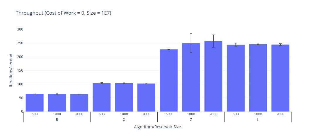
It varies the size of the reservoir, the size of the input, and uses Blackhole.consumeCPU to roughly simulate the cost of doing some actual work to produce sampled values, in order to demonstrate that if the application logic is slow enough, fast sampling algorithms aren’t very interesting.
    @Benchmark
    public AlgorithmR R(RState state) {
        AlgorithmR r = state.algorithmR;
        for (double v : state.data) {
            Blackhole.consumeCPU(state.costOfWork);
            r.add(v);
        }
        return r;
    }


    @Benchmark
    public AlgorithmX X(XState state) {
        AlgorithmX x = state.algorithmX;
        for (double v : state.data) {
            Blackhole.consumeCPU(state.costOfWork);
            x.add(v);
        }
        return x;
    }

    @Benchmark
    public AlgorithmZ Z(ZState state) {
        AlgorithmZ z = state.algorithmZ;
        for (double v : state.data) {
            Blackhole.consumeCPU(state.costOfWork);
            z.add(v);
        }
        return z;
    }

    @Benchmark
    public AlgorithmL L(LState state) {
        AlgorithmL l = state.algorithmL;
        for (double v : state.data) {
            Blackhole.consumeCPU(state.costOfWork);
            l.add(v);
        }
        return l;
    }
When the cost of producing the samples is essentially free, both of Vitter’s algorithms are orders of magnitude better than Algorithm R.
Once the work is more expensive (100 tokens) there is no discernible difference. This is unsurprising.
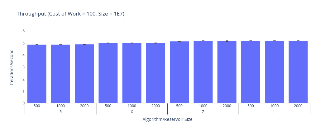
I doubt that the performance analysis from the 80s is remotely relevant today, and there are probably modern day tricks to speed Algorithm X up.
Testing
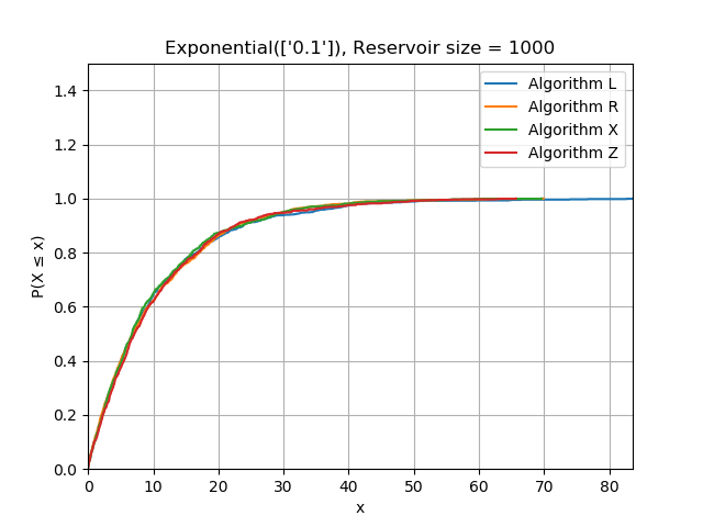
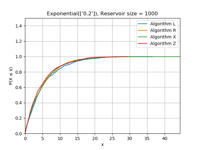
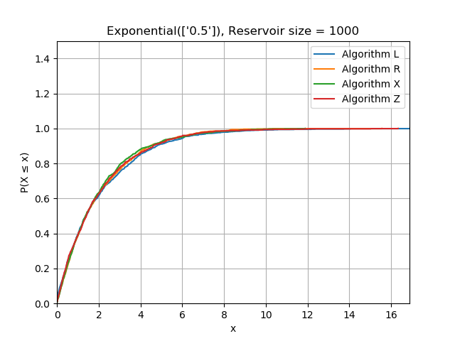
It looks like algorithms X and Z are much faster than R, but are they correct? Testing this is a bit more complicated than writing a typical unit test because we need to test statistical properties rather than literal values. As a basic sanity check, I generated exponentially distributed data, sorted it, and verified I could reproduce the maximum likelihood estimator within a loose tolerance from the reservoir. Sorting the data will reveal bias towards the start or end of the stream by producing a different distribution function.
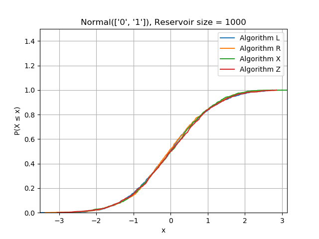
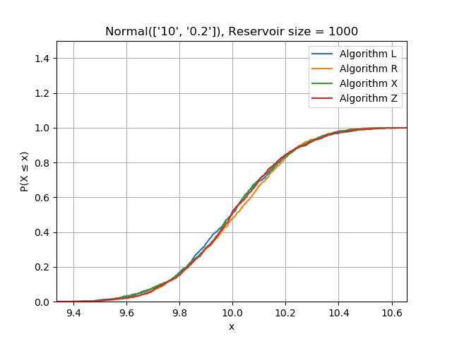
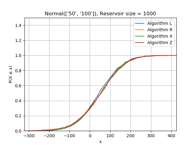
I also generated data from a range of different distributions and plotted the CDF of the contents of each reservoir having seen the same data. This is a complicated topic which I will treat more seriously in another post.
References
Further Reading
- An Efficient Algorithm for Sequential Random Sampling Vitter’s later work, which recommended Algorithm D when $N$ is known.
- Very Fast Reservoir Sampling a good blog post, complementary to this post. Written much later than Vitter’s work but reportedly independently of An Efficient Algorithm for Sequential Random Sampling.