Maximum Likelihood Estimation
Feedback on these posts is welcome and solicited. If you find mistakes, corrections can be made by pull request at GitHub.
Suppose you want to model a system in order to gain insight about its behaviour. Having collected some measurements of the state variables of your system, you want to infer their distribution so you can generate input for a system simulation. With some insight it may be possible to guess the family of distribution the data belongs to, in which case it is enough to find the distribution parameters which best fit the observations. This process is known as statistical inference. This post revisits maximum likelihood estimation (MLE), a simple inference method.
Eyeball Statistics
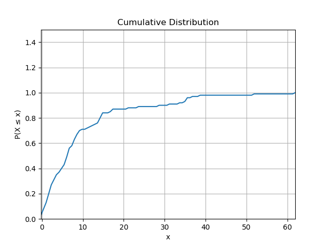
Here’s the raw data we want to determine the distribution of, which might correspond to inter-arrival times of some messages, measured in microseconds.
[ 1.66  2.69 13.66  7.02  8.00  4.28  2.37 23.66 35.63  1.79  8.38  2.71
 61.63  8.09  3.26 14.75  0.56  1.04 34.87 36.71  6.14  0.63  9.64 15.30
  8.62 35.39 15.06  8.26  7.02 14.56 14.66 15.20  7.77 12.39 38.40  1.77
  5.86  4.43 16.83  0.07  1.51 21.13 11.01  3.26  3.41  0.66  8.62  1.86
  4.00 11.93  5.32  1.25  1.67  6.83  5.29 33.66 14.16  2.26  8.81 17.54
  6.00  3.52  3.94  9.82  8.23  6.76  2.50  6.52  9.33  7.14 35.21 31.35
  3.52  0.17  5.22  9.32 17.70  6.89  0.18  2.61  6.17  1.50 14.60  6.66
  0.49  5.49  7.78 13.12  6.01  0.44 51.66  2.44  1.98  1.21  3.00  2.12
  6.56  5.77  8.53 28.80]
With a little bit of python scripting we can calculate the cumulative frequency.
from scipy import stats

cdf = stats.cumfreq(samples, numbins=len(samples))
After normalising we can plot the cumulative distribution, which is noisy because we don’t have much data.
It’s likely we can make an educated guess about the distribution of the data, so we can know which parameters we are trying to fit. The guess about the family of distribution may be driven by experience or convenience, but for some distributions there are tests which can be applied to the data. Validating the guess is beyond the scope of this post.
We have heard that uncorrelated arrival times tend to be exponentially distributed, so guess that this is the case for the measurements. The distribution function is specified as:
\[F(x; \lambda) = 1 - \exp(-\lambda x), x \geq 0\]So we could just plot that function for a range of values of $\lambda$ and see which is closest to the data.
import numpy as np

t = np.arange(0, 100, 0.01)
y1 = np.vectorize(lambda l: 1.0 - math.exp(-l * 0.05))(t)
y2 = np.vectorize(lambda l: 1.0 - math.exp(-l * 0.1))(t)
y3 = np.vectorize(lambda l: 1.0 - math.exp(-l * 0.15))(t)
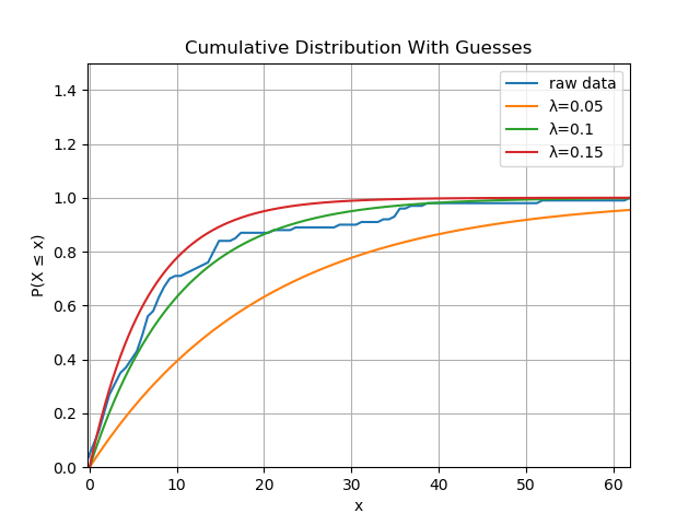
The blue line is quite close to the green line, where we guessed $\lambda$ was 0.1, and is always between the red and orange lines, so $\lambda$ must be between 0.05 and 0.15. This process is as intuitive as it is manual; it’s better to have a systematic way of doing this. Moreover, the exponential distribution is a very simple distribution with one parameter, but there are plenty of two and three parameter distributions. Comparing curves won’t scale in the number of parameters.
How to automate this process and generalise to higher dimensional parameter spaces? Parametric inference is essentially a search procedure in parameter space. Given a sample as input, the search procedure’s objective is to find the point in parameter space which minimises the “distance” between the sample and CDF described by the parameters. This is what we are doing by “eyeballing” distributions: vary the parameters until a curve looks close to the data.
I don’t know for sure that a search guided by a distance measure between sample and CDF is an awful idea, but it’s certainly not what’s taught in statistical inference courses. At the very least, it seems problematic - in terms of the significance of two curves being “close” - that the CDFs converge; measurements drawn from a distribution with a very fat tail are indistinguishable from freak measurements drawn from a thin-tailed distribution, if we don’t consider the plausibility of having made the measurement.
I am as guilty - or even more guilty - as anyone else not working as a statistician of relying on “eyeball statistics”, despite having been taught better at some point.
Maximum Likelihood Estimation
Rather than minimising the distance between sample and curve, MLE selects parameters by maximising the likelihood - as opposed to probability - of the sample being drawn from the distribution associated with the parameters. I never really appreciated the difference between likelihood and probability as a student, except that probability is defined in terms of a probability space, which assumes an assignment of probabilities to events. This makes it problematic to go backwards because this assignment is what we are trying to infer. In any case, likelihood is practically the same thing as probability; the likelihood function behaves like a joint probability density function.
We have already assumed that all the samples are from the same distribution, but will also assume that the samples are independent because dependent events make joint densities complicated. This simplifying assumption is not necessary, but is a common one. When the events are independent the joint density can be expressed as the product of the marginal densities, which makes the maths easier to do.
This is quite a simplifying assumption: consider the independence of inter-arrival times with failures and retries.
Given the i.i.d. assumption, the likelihood function of the parameters $\vec{\theta}$ and the sample $ \vec{x}$ is written as follows:
\[L(\vec{\theta}; \vec{x}) = \prod_i \mathrm{pdf}(\vec{\theta}; x_i)\]Maximising it means computing the partial derivative for each parameter, and intersecting the zero roots of the derivatives. In practice, this is too difficult to do for two reasons:
- Computing the partial derivative might be difficult or even analytically impossible depending on the probability density function.
- Computing the partial derivative often is analytically impossible, so it is done numerically (or by automatic differentiation). The product of many small numbers is very small and there is a risk of underflow.
For these reasons, along with the fact that many standard distributions have exponential terms, the natural logarithm of the likelihood function is maximised. The natural logarithm is a good choice because it is monotonic so composition with it does not change the locations of the maxima. Happily, the transformation maps multiplications to additions, which mollifies the issue of numerical underflow.
However, inferring parameters from a sample analytically is relatively straightforward for standard distributions. I remember inferring normal distribution parameters being a ten minute exam question. It is especially easy for the exponential distribution because there is only one parameter making the calculus easy and the intersection a no-op.
The first mathematical expression given was the cumulative distribution function, which is actually the integral of the density function. Here’s the probability density function:
\[\mathrm{pdf}(\lambda; x) = \lambda \exp(-\lambda x), x \geq 0\]So the likelihood function is:
\[L(\lambda; \vec{x}) = \prod_i \lambda \exp(-\lambda x_i)\]Which simplifies to:
\[L(\lambda; \vec{x}) = \lambda^n \exp(-\lambda (\sum_i x_i)\]It’s easier to differentiate the log likelihood which removes the exponential term:
\[l(\lambda; \vec{x}) = n \ln \lambda - \lambda \sum_i x_i\]Differentiating with respect to $\lambda$, the maximum likelihood must be specified by:
\[\frac{n}{\lambda} - \sum_i x_i = 0\]Or:
\[\lambda = \frac{n}{\sum_i x_i}\]Notably, this is the reciprocal of both the model and observed mean ($1/\lambda$ is the first moment of the exponential distribution).
If this had been the normal distribution, with mean $\mu$ and standard deviation $\sigma$, the procedure would have been a little bit more complicated. The log likelihood would have been differentiated with respect to $\mu$ and $\sigma$ separately, leaving simultaneous equations to solve. For other distributions, this process requires numerical solution.
Sanity Check
Applying the expression obtained for $\lambda$ to the data we get close to 0.1: the code below prints 0.0975.
lambda_estimate = samples.size / np.sum(samples)
print("{:.4f}".format(lambda_estimate))
This is reassuring because the sample data was actually generated by a random number generator with $\lambda = 0.1$!
import math
from random import random

def exp_rv(rate):
    return (-1.0 / rate) * math.log(random())


def generate(rate, count):
    return np.vectorize(lambda _: exp_rv(rate))(np.arange(count))


samples = generate(0.1, 100)
However, it’s not exactly 0.1: does it get better with more data and are we guaranteed to get a sensible estimate?
intensity = 0.1
for n in range(1, 7):
    size = pow(10, n)
    print(size / np.sum(generate(intensity, size)))
The snippet above prints output which seems to suggest the estimate gets better with more data, so long as the data really does conform to the distribution:
0.12447329039974349
0.08998606757933628
0.10439439508646252
0.09843159954973514
0.1000660471700133
0.10000469172954365
The cumulative distribution functions inferred from the data get closer to the model as the sample size increases.
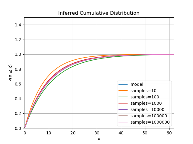
The estimator is actually proven to be consistent for all parametric distributions, that is, the estimates converge almost surely to the model parameters. So, assuming you have enough data satisfying the assumptions, this is a robust technique for determining the distribution.
However, it’s easy to imagine degenerate cases where MLE as performed in this post probably won’t work:
- The measurements aren’t independent, e.g. retries.
- The measurements aren’t identically distributed: the same service may handle traffic from different sources behaving differently.
- The measurements don’t conform to a nice distribution: imagine there are sporadic STW GC pauses delaying the recording of some arrival times.