RangeBitmap - How range indexes work in Apache Pinot
Suppose you have an unsorted array of numeric values and need to find the set of indexes of all the values which are within a range. The range predicate will be evaluated many times, so any time spent preprocessing will be amortised, and non-zero spatial overhead is expected. If the data were sorted, this would be very easy, but the indexes of the values have meaning so the data cannot be sorted. To complicate the problem slightly, the set of indexes must be produced in sorted order.
These are the requirements for a range index in a column store, where the row indexes implicitly link values stored separately in different columns. The purpose of a range index is to accelerate a query like the one below which identifies all spans in a time window where the duration exceeds 10ms (in nanoseconds):
select
  traceId,
  spanId,
  operationName
from
  spans
where
  duration > 10000000
  and timestamp between '2022-03-06 02:00:00.000'
  and '2022-03-06 03:00:00.000'
How can the spans be indexed to make this query as fast as it can be? Different databases solve this problem in different ways, but the context of this post is a column store like Apache Pinot.
It’s unusual for there to be only one important class of query, so other constraints need to be taken into account. The query above for slow spans isn’t the only query that needs to be fast, queries like the one below to compute the time spent in each operation of a trace also need to execute quickly:
select
  serviceName,
  operationName,
  count(*),
  sum(duration)
from
  spans
where
  traceId = 1234578910
group by
  serviceName,
  operationName
Apache Pinot tables consist of segments which usually correspond to the data ingested from a stream within a time window, and will generally have the same implicit partitioning as the stream. Segments have a columnar layout, and contain their indexes, metadata, and other data structures. Segments are independent of each other and all data structures are scoped to their segment; data is sorted within the scope of a segment and not globally, and so on.
A Pinot cluster consists of four different classes of service which have different responsibilities, of which two are relevant to how to optimise this query. Servers are responsible for querying segments, they know how to read the segment format, load indexes, prune (avoid querying) and query the segments and merge segment-level query results into server-level query results. Brokers are responsible for routing queries to servers and merging server-level results, they can perform some amount of segment pruning to protect the servers’ resources.
The second query needing to be fast imposes constraints on what can be done to optimise the first query.
Firstly, brokers can use knowledge of segment partitioning to optimise query routing.
If we need the second query to be fast, we should partition on traceId which limits the number of servers the broker need to route the query to.
Unless the trace’s duration exceeds the time taken to produce one segment (which may happen when tracing batch systems), all the spans in a trace should fit in a single segment, so partitioning by traceId should mean only a single segment need be queried.
This means that the first query (find all the slow spans in the last hour) will not be able to use partitioning to prune segments and the query will be routed to all servers.
The second query will also need an index on traceId to be efficient because a typical segment will contain millions of rows, and scanning all these rows will be too slow.
Choosing an appropriate index requires some knowledge of the data (though this decision can be automated given representative sample data).
In case you are unfamiliar with tracing, traceId and spanId are high cardinality attributes and there is a hierarchical relationship between spans and traces: a trace is a collection of spans.
We should expect that traces last at most minutes and consist of fewer than 1000 spans in the typical case.
Pinot has several types of index, but the choice here would be between a sorted index and an inverted index. Sorted indexes offer the best space/time tradeoff of Pinot’s indexes but, unsurprisingly, a sorted index can only be applied to a sorted column, and only one column can be sorted. This makes the choice of sorted column one of the biggest decisions when designing a Pinot table.
Given the hierarchical relationship between traceId and spanId, and an expectation that most traces will contain far fewer than 1000 spans, sorting on traceId indexes spanId for free because a scan for spanId would inspect only spans within the same trace.
Creating an inverted index on traceId is a possibility, but it would have quite high cardinality: if there are 10M spans in a segment, and 100 spans per trace, then there would be 100k postings lists.
Moreover, the performance of the aggregation in the second query depends on locality, which sorting improves.
In this case, the case for sorting by traceId probably trumps sorting by duration or timestamp.
Fortunately, the timestamp filter can be used to prune segments if it is configured as the time column.
Segments have metadata including the minimum and maximum value of the time column, and these time boundary values can be used to eliminate segments before querying them.
The filter timestamp between '2022-03-06 02:00:00.000' and '2022-03-06 03:00:00.000' narrows the segments to query down to those with boundary values which intersect with the hour specified by the query.
Assuming that each segment corresponds to 3 hours of ingested events within its partition, pruning by time boundary cuts the number of segments which need to be pruned from all segments ever to at most twice the number of partitions.
However, within each of the unpruned segments, there are still millions of records which need to be filtered to find the slow spans in the time range, and the rows within the segments aren’t sorted by timestamp.
All of this is enough to justify the existence of a range index in a system like Pinot.
This post is about the design and implementation of RangeBitmap, a data structure which powers Pinot’s new range indexes.
- Implementing a Range Index
- Bit slicing
- RangeBitmap design
- Usage in Apache Pinot
- Links:
Implementing a Range Index
Zooming into the data now, imagine you have an array of durations like those below, which are all small numbers for the sake of simplicity:
$[10, 3, 15, 0, 0, 1, 5, 6, 2, 1, 12, 14, 3, 9, 11]$
We want to get the row indexes of the values which satisfy predicates so attributes at the same indexes can be selected. We also want the sets to be sorted so scans over other columns are sequential which is more efficient than traversing in random order. From the list above we would want the following outputs for each of the predicates below:
| predicate | expected output |
|---|---|
| $x < 3$ | $ \{3, 4, 5, 8, 9 \} $ |
| $x < 10$ | $ \{ 1, 3, 4, 5, 6, 7, 8, 9, 12, 13 \}$ |
| $x > 5$ | $ \{0, 2, 7, 10, 11, 13, 14 \}$ |
| $2 < x < 10$ | $ \{ 1, 6, 7, 12, 13 \}$ |
| $5 < x < 10$ | $ \{ 7, 13 \}$ |
Or represented as bitmaps which can be iterated over we would have the following:
| value | $< 3$ | $< 10$ | $> 5$ |
|---|---|---|---|
| 10 | 0 | 0 | 1 |
| 3 | 0 | 1 | 0 |
| 15 | 0 | 0 | 1 |
| 0 | 1 | 1 | 0 |
| 0 | 1 | 1 | 0 |
| 1 | 1 | 1 | 0 |
| 5 | 0 | 1 | 0 |
| 6 | 0 | 1 | 1 |
| 2 | 1 | 1 | 0 |
| 1 | 1 | 1 | 0 |
| 12 | 0 | 0 | 1 |
| 14 | 0 | 0 | 1 |
| 3 | 0 | 1 | 0 |
| 9 | 0 | 1 | 1 |
| 11 | 0 | 0 | 1 |
Representing the array indexes as bitmaps is beneficial because they can be combined with bitmaps obtained from other indexes to satisfy complex filter constraints without needing indexes which themselves can understand every filter constraint. The following filters should be pushed down into a range index for efficiency reasons, but demonstrate how to build a double bounded range from two single bounded ranges:
| value | $< 10$ | $> 5$ | $5 < x < 10$ |
|---|---|---|---|
| 10 | 0 | 1 | 0 & 1 = 0 |
| 3 | 1 | 0 | 1 & 0 = 0 |
| 15 | 0 | 1 | 0 & 1 = 0 |
| 0 | 1 | 0 | 1 & 0 = 0 |
| 0 | 1 | 0 | 1 & 0 = 0 |
| 1 | 1 | 0 | 1 & 0 = 0 |
| 5 | 1 | 0 | 1 & 0 = 0 |
| 6 | 1 | 1 | 1 & 1 = 1 |
| 2 | 1 | 0 | 1 & 0 = 0 |
| 1 | 1 | 0 | 1 & 0 = 0 |
| 12 | 0 | 1 | 0 & 1 = 0 |
| 14 | 0 | 1 | 0 & 1 = 0 |
| 3 | 1 | 0 | 1 & 0 = 0 |
| 9 | 1 | 1 | 1 & 1 = 1 |
| 11 | 0 | 1 | 0 & 1 = 0 |
Pinot’s indexes use RoaringBitmap to represent filters, so the range index will produce a RoaringBitmap too.
Bit slicing
The algorithm used to do range evaluations is described in the 1998 paper Bitmap Index Design and Evaluation. This algorithm has been used at least twice before: the paper mentions that SybaseIQ used it in the 90s, and pilosa also implemented it in the last decade. To understand it, first look at the binary layout of the numbers in the example, which have all been chosen to be representable in 4 bits to limit the number of columns I need to write.
| value | bit 3 | bit 2 | bit 1 | bit 0 |
|---|---|---|---|---|
| 10 | 1 | 0 | 1 | 0 |
| 3 | 0 | 0 | 1 | 1 |
| 15 | 1 | 1 | 1 | 1 |
| 0 | 0 | 0 | 0 | 0 |
| 0 | 0 | 0 | 0 | 0 |
| 1 | 0 | 0 | 0 | 1 |
| 5 | 0 | 1 | 0 | 1 |
| 6 | 0 | 1 | 1 | 0 |
| 2 | 0 | 0 | 1 | 0 |
| 1 | 0 | 0 | 0 | 1 |
| 12 | 1 | 1 | 0 | 0 |
| 14 | 1 | 1 | 1 | 0 |
| 3 | 0 | 0 | 1 | 1 |
| 9 | 1 | 0 | 0 | 1 |
| 11 | 1 | 0 | 1 | 1 |
The columns can be used to evaluate filters. For instance, the numbers greater than seven all have a bit in the leftmost column. Looking at the leftmost column would be enough to evaluate $x > 7$ but not $x > 8$ which also requires at least one bit in the three columns to the right. This gets coarser as the number of bits in the numbers increases so trying to post-filter wouldn’t scale well.
To arrive at an algorithm, each column can be range encoded so that there are two slices for each column: a bit is set in the $i$th slice if the bit is less than or equal to $i \in \{0, 1\}$.
| value | predicate | bit 3 | bit 2 | bit 1 | bit 0 |
|---|---|---|---|---|---|
| 10 | $\leq 0$ | 0 | 1 | 0 | 1 |
| $\leq 1$ | 1 | 1 | 1 | 1 | |
| 3 | $\leq 0$ | 1 | 1 | 0 | 0 |
| $\leq 1$ | 1 | 1 | 1 | 1 | |
| 15 | $\leq 0$ | 0 | 0 | 0 | 0 |
| $\leq 1$ | 1 | 1 | 1 | 1 | |
| 0 | $\leq 0$ | 1 | 1 | 1 | 1 |
| $\leq 1$ | 1 | 1 | 1 | 1 | |
| 0 | $\leq 0$ | 1 | 1 | 1 | 1 |
| $\leq 1$ | 1 | 1 | 1 | 1 | |
| 1 | $\leq 0$ | 1 | 1 | 1 | 0 |
| $\leq 1$ | 1 | 1 | 1 | 1 | |
| 5 | $\leq 0$ | 1 | 0 | 1 | 0 |
| $\leq 1$ | 1 | 1 | 1 | 1 | |
| 6 | $\leq 0$ | 1 | 0 | 0 | 1 |
| $\leq 1$ | 1 | 1 | 1 | 1 | |
| 2 | $\leq 0$ | 1 | 1 | 0 | 1 |
| $\leq 1$ | 1 | 1 | 1 | 1 | |
| 1 | $\leq 0$ | 1 | 1 | 1 | 0 |
| $\leq 1$ | 1 | 1 | 1 | 1 | |
| 12 | $\leq 0$ | 0 | 0 | 1 | 1 |
| $\leq 1$ | 1 | 1 | 1 | 1 | |
| 14 | $\leq 0$ | 0 | 0 | 0 | 1 |
| $\leq 1$ | 1 | 1 | 1 | 1 | |
| 3 | $\leq 0$ | 1 | 1 | 0 | 0 |
| $\leq 1$ | 1 | 1 | 1 | 1 | |
| 9 | $\leq 0$ | 0 | 1 | 1 | 0 |
| $\leq 1$ | 1 | 1 | 1 | 1 | |
| 11 | $\leq 0$ | 0 | 1 | 0 | 0 |
| $\leq 1$ | 1 | 1 | 1 | 1 |
Of course, a bit can only ever be $\leq 1$ because they only take two values, so the second slice is redundant and the table becomes:
| value | bit 3 | bit 2 | bit 1 | bit 0 |
|---|---|---|---|---|
| 10 | 0 | 1 | 0 | 1 |
| 3 | 1 | 1 | 0 | 0 |
| 15 | 0 | 0 | 0 | 0 |
| 0 | 1 | 1 | 1 | 1 |
| 0 | 1 | 1 | 1 | 1 |
| 1 | 1 | 1 | 1 | 0 |
| 5 | 1 | 0 | 1 | 0 |
| 6 | 1 | 0 | 0 | 1 |
| 2 | 1 | 1 | 0 | 1 |
| 1 | 1 | 1 | 1 | 0 |
| 12 | 0 | 0 | 1 | 1 |
| 14 | 0 | 0 | 0 | 1 |
| 3 | 1 | 1 | 0 | 0 |
| 9 | 0 | 1 | 1 | 0 |
| 11 | 0 | 1 | 0 | 0 |
This mapping is easy to perform because it’s just the logical complement of the input values masked by how many bits we care about, so x -> ~x & 0xF in this case.
Now there is a bitset in each slice:
| 0 | 1 | 2 | 3 |
|---|---|---|---|
100110011011000 |
000111100110010 |
110111001100111 |
010111111100100 |
Performing a transposition like this incurs no spatial overhead, and can end up smaller than storing the data itself if the values have many leading zeros allowing slices to be pruned, especially if bitmap compression is applied to the columns.
A predicate $x \leq t$ can be evaluated against the slices, assuming $n$ rows were indexed as follows:
- Assume all rows match, initialise bitmap
stateto $[0, n)$, that is set every bit between 0 and $n$. - for each bit in
t:- if
t[i]is set, setstate=state | slices[i]- These bits need to be included in the result because they mean this coefficient in the input was less than the same coefficient of the threshold
- if
t[i]is not set, setstate=state & slices[i]- Bits absent in the slice need to be removed because it means the bit was present
- if
To evaluate an $x > t$ predicate, just take the logical complement of the result of an $x \leq t$ predicate. Predicates $x < t$ or $x \geq t$ can be evaluated by adding or subtracting 1 from the threshold and evaluating a $x \leq t$ or $x > t$ predicate respectively. A double ended range $t \leq x \leq u$ can be evaluated by intersecting $x > t$ and $x \leq u$.
This algorithm has strengths and weaknesses. Firstly, it should be clear it can’t compete with the potentialities of sorting the data: binary search over run-length encoded values or even the raw data has lower time complexity. The complexity is linear in the product of the number of rows and the number of slices, so evaluation time depends on the largest value in the data set. However, logical operations between bitmaps are very efficient and can be vectorised, so hundreds of rows can be evaluated in a handful of CPU instructions. Space is saved by storing the row indexes implicitly in the positions of the bits (and this is improved by the compression explained later), and it automatically produces sorted outputs. The various tree data structures which could also solve this problem can’t compress the row indexes (though some can compress the values) and would all need to sort the row indexes after evaluating the predicate, which prevents lazy evaluation.
Generalisation to higher bases
Any number can be expressed as the coefficients of a polynomial with base $b$, binary numbers just have coefficients 0 or 1. Other bases can be chosen, which create space/time tradeoffs best visualised by considering the representations of numbers in different bases:
| base | representation |
|---|---|
| 2 | 111010110111100110100010101 |
| 3 | 22121022020212200 |
| 4 | 13112330310111 |
| 8 | 726746425 |
| 10 | 123456789 |
| 16 | 75bcd15 |
In base-2, a large number 123456789 has 27 digits, but only one slice per digit, so the range encoding operation is lightning fast and has no write-amplification. At the other end of the spectrum, in base-16 there are only 7 digits but 15 slices per digits. Reducing the number of digits reduces the number of bitmap operations which need to be performed, but increase spatial overhead and write amplification. Bitmap Index Design and Evaluation explores this tradeoff (see here for implementations).
Example
This is an example of how to evaluate the predicate $x \leq 9$ or $x < 10$ against a 4-bit base-2 index.
There is a table for each step of the algorithm:
- The far left column in each has the value as encountered in the data, the next four columns represent the values stored in the index; these columns never change.
- The next column represents the state bitmap, which changes on each step of the algorithm (and if it doesn’t, this step should be eliminated if it can be detected).
- The final two columns represent the target, the bitmap we know we want to have produced once the algorithm has terminated, and whether the state bitmap is currently accurate.
- The far right column should give the intuition that the algorithm doesn’t converge to a solution and randomly flips bits depending on what’s in the slice. In this example, the hamming distance between the state and the solution only increases until the last step.
- The bold column is the slice being operated on.
The threshold 9 in binary is 1001, so the first and last slices will be united, and the middle slices will be intersected.
Initialise state
| value | slice 3 | slice 2 | slice 1 | slice 0 | state | target | |
|---|---|---|---|---|---|---|---|
| 10 | 0 | 1 | 0 | 1 | 1 | 0 | ❌ |
| 3 | 1 | 1 | 0 | 0 | 1 | 1 | ✔️ |
| 15 | 0 | 0 | 0 | 0 | 1 | 0 | ❌ |
| 0 | 1 | 1 | 1 | 1 | 1 | 1 | ✔️ |
| 0 | 1 | 1 | 1 | 1 | 1 | 1 | ✔️ |
| 1 | 1 | 1 | 1 | 0 | 1 | 1 | ✔️ |
| 5 | 1 | 0 | 1 | 0 | 1 | 1 | ✔️ |
| 6 | 1 | 0 | 0 | 1 | 1 | 1 | ✔️ |
| 2 | 1 | 1 | 0 | 1 | 1 | 1 | ✔️ |
| 1 | 1 | 1 | 1 | 0 | 1 | 1 | ✔️ |
| 12 | 0 | 0 | 1 | 1 | 1 | 0 | ❌ |
| 14 | 0 | 0 | 0 | 1 | 1 | 0 | ❌ |
| 3 | 1 | 1 | 0 | 0 | 1 | 1 | ✔️ |
| 9 | 0 | 1 | 1 | 0 | 1 | 1 | ✔️ |
| 11 | 0 | 1 | 0 | 0 | 1 | 0 | ❌ |
Union with slice 0
Perform a destructive logical union between the first slice and the state, modifying the state bitmap.
| value | slice 3 | slice 2 | slice 1 | slice 0 | state | target | |
|---|---|---|---|---|---|---|---|
| 10 | 0 | 1 | 0 | 1 | 1 | 0 | ❌ |
| 3 | 1 | 1 | 0 | 0 | 1 | 1 | ✔️ |
| 15 | 0 | 0 | 0 | 0 | 1 | 0 | ❌ |
| 0 | 1 | 1 | 1 | 1 | 1 | 1 | ✔️ |
| 0 | 1 | 1 | 1 | 1 | 1 | 1 | ✔️ |
| 1 | 1 | 1 | 1 | 0 | 1 | 1 | ✔️ |
| 5 | 1 | 0 | 1 | 0 | 1 | 1 | ✔️ |
| 6 | 1 | 0 | 0 | 1 | 1 | 1 | ✔️ |
| 2 | 1 | 1 | 0 | 1 | 1 | 1 | ✔️ |
| 1 | 1 | 1 | 1 | 0 | 1 | 1 | ✔️ |
| 12 | 0 | 0 | 1 | 1 | 1 | 0 | ❌ |
| 14 | 0 | 0 | 0 | 1 | 1 | 0 | ❌ |
| 3 | 1 | 1 | 0 | 0 | 1 | 1 | ✔️ |
| 9 | 0 | 1 | 1 | 0 | 1 | 1 | ✔️ |
| 11 | 0 | 1 | 0 | 0 | 1 | 0 | ❌ |
This step didn’t actually change the state bitmap, and could have been eliminated by checking if the LSB is set.
Intersection with slice 1
Perform a destructive logical intersection between the second slice and the state bitmap, modifying the state bitmap.
| value | slice 3 | slice 2 | slice 1 | slice 0 | state | target | |
|---|---|---|---|---|---|---|---|
| 10 | 0 | 1 | 0 | 1 | 0 | 0 | ✔️ |
| 3 | 1 | 1 | 0 | 0 | 0 | 1 | ❌ |
| 15 | 0 | 0 | 0 | 0 | 0 | 0 | ✔️ |
| 0 | 1 | 1 | 1 | 1 | 1 | 1 | ✔️ |
| 0 | 1 | 1 | 1 | 1 | 1 | 1 | ✔️ |
| 5 | 1 | 0 | 1 | 0 | 1 | 1 | ✔️ |
| 1 | 1 | 1 | 1 | 0 | 1 | 1 | ✔️ |
| 6 | 1 | 0 | 0 | 1 | 0 | 1 | ❌ |
| 2 | 1 | 1 | 0 | 1 | 0 | 1 | ❌ |
| 1 | 1 | 1 | 1 | 0 | 1 | 1 | ✔️ |
| 12 | 0 | 0 | 1 | 1 | 1 | 0 | ❌ |
| 14 | 0 | 0 | 0 | 1 | 0 | 0 | ✔️ |
| 3 | 1 | 1 | 0 | 0 | 0 | 1 | ❌ |
| 9 | 0 | 1 | 1 | 0 | 1 | 1 | ❌ |
| 11 | 0 | 1 | 0 | 0 | 0 | 0 | ✔️ |
Intersection with slice 2
Perform a destructive logical intersection between the third slice and the state bitmap, modifying the state bitmap.
| value | slice 3 | slice 2 | slice 1 | slice 0 | state | target | |
|---|---|---|---|---|---|---|---|
| 10 | 0 | 1 | 0 | 1 | 0 | 0 | ✔️ |
| 3 | 1 | 1 | 0 | 0 | 0 | 1 | ❌ |
| 15 | 0 | 0 | 0 | 0 | 0 | 0 | ✔️ |
| 0 | 1 | 1 | 1 | 1 | 1 | 1 | ✔️ |
| 0 | 1 | 1 | 1 | 1 | 1 | 1 | ✔️ |
| 5 | 1 | 0 | 1 | 0 | 0 | 1 | ❌ |
| 1 | 1 | 1 | 1 | 0 | 1 | 1 | ✔️ |
| 6 | 1 | 0 | 0 | 1 | 0 | 1 | ❌ |
| 2 | 1 | 1 | 0 | 1 | 0 | 1 | ❌ |
| 1 | 1 | 1 | 1 | 0 | 1 | 1 | ✔️ |
| 12 | 0 | 0 | 1 | 1 | 0 | 0 | ✔️ |
| 14 | 0 | 0 | 0 | 1 | 0 | 0 | ✔️ |
| 3 | 1 | 1 | 0 | 0 | 0 | 1 | ❌ |
| 9 | 0 | 1 | 1 | 0 | 1 | 1 | ✔️ |
| 11 | 0 | 1 | 0 | 0 | 0 | 0 | ✔️ |
Union with slice 3 and terminate
Perform a destructive logical union between the fourth slice and the state bitmap, modifying the state bitmap.
| value | slice 3 | slice 2 | slice 1 | slice 0 | state | target | |
|---|---|---|---|---|---|---|---|
| 10 | 0 | 1 | 0 | 1 | 0 | 0 | ✔️ |
| 3 | 1 | 1 | 0 | 0 | 1 | 1 | ✔️ |
| 15 | 0 | 0 | 0 | 0 | 0 | 0 | ✔️ |
| 0 | 1 | 1 | 1 | 1 | 1 | 1 | ✔️ |
| 0 | 1 | 1 | 1 | 1 | 1 | 1 | ✔️ |
| 5 | 1 | 0 | 1 | 0 | 1 | 1 | ✔️ |
| 1 | 1 | 1 | 1 | 0 | 1 | 1 | ✔️ |
| 6 | 1 | 0 | 0 | 1 | 1 | 1 | ✔️ |
| 2 | 1 | 1 | 0 | 1 | 1 | 1 | ✔️ |
| 1 | 1 | 1 | 1 | 0 | 1 | 1 | ✔️ |
| 12 | 0 | 0 | 1 | 1 | 0 | 0 | ✔️ |
| 14 | 0 | 0 | 0 | 1 | 0 | 0 | ✔️ |
| 3 | 1 | 1 | 0 | 0 | 1 | 1 | ✔️ |
| 9 | 0 | 1 | 1 | 0 | 1 | 1 | ✔️ |
| 11 | 0 | 1 | 0 | 0 | 0 | 0 | ✔️ |
There are no more slices so the algorithm terminates here.
Optimisations
The algorithm’s time complexity is super-linear, depending on both the number of indexed rows and how many slices are present in the indexed values. This means that every slice which doesn’t need to be operated on (the first step in the example above was redundant) should be eliminated.
There are various fast-forwarding optimisations which eliminate bitmap operations between slices at the start of the evaluation. Some of these depend on the threshold:
- Evaluating the result for the first slice has redundancy: if the LSB is set in the threshold, the first union is redundant.
Similarly, if it isn’t set, the
statebitmap can be initialised to the values of the first slice; initialising to[0, max)beforehand is redundant. - If there is a run of $k$ set bits starting from 0, all $k$ operations can be eliminated.
Others depend on the data:
- If there is an empty slice at position $k$ and the bit $k$ is absent from the threshold $x$, the
statebitmap will be empty afterwards. All $k$ operations can be replaced by just settingstateto $\emptyset$. - If there is a full slice at position $k$ and the bit $k$ is present in the threshold $x$, the
statebitmap will be full afterwards, so all $k$ operations can be replaced by settingstateto $[0, max)$
The example above was for a 4-bit index, but arbitrary size numbers (64 bits is an artificial limit) can be indexed in theory, given a choice of a maximum value. However, allocating capacity for values much larger than the largest indexed value leads to unnecessary slices and slower evaluations. Knowing the maximum value reduces the number of slices which need to be operated on.
Similarly, if the minimum value is large, subtracting it from each value reduces the number of slices by a factor of $\log_2(x_{min})$. This is especially important for indexing timestamps, where the minimum timestamp in a data set will often have a large offset from 1970-01-01. At the time of writing, the unix epoch time is $1646510472$, and a collection of timestamps over the next 24 hours would fall in the range $[1646510472, 1646596872]$. The number of slices required to encode this range would be $ \lceil \log_2( 1646596872 ) \rceil = 31$, whereas to index $[0, 1646596872 - 1646510472]$ or $[0, 86400]$ only $ \lceil \log_2(86400) \rceil = 17$ slices are required, which roughly halves the evaluation time.
Horizontal and Vertical Evaluations
An important implementation choice is whether to operate on an entire slice at a time (vertically) or across a small horizontal section of all slices producing a section of the final result (horizontally).
In the step by step example of the algorithm above, the evaluation was vertical. Instead, let’s say we perform all four operations two rows at a time (recall that to evaluate $v \leq 9$ there was a union followed by two intersections and a final union) and append the partial result to an output incrementally. The evaluation would proceed as follows:
OR slice 0, AND slice 1, AND slice 2, OR slice 3, append result for rows 0, 1
| value | slice 3 | slice 2 | slice 1 | slice 0 | state | target | |
|---|---|---|---|---|---|---|---|
| 10 | 0 | 1 | 0 | 1 | 0 | 0 | ✔️ |
| 3 | 1 | 1 | 0 | 0 | 1 | 1 | ✔️ |
| 15 | 0 | 0 | 0 | 0 | - | 0 | ❓ |
| 0 | 1 | 1 | 1 | 1 | - | 1 | ❓️ |
| 0 | 1 | 1 | 1 | 1 | - | 1 | ❓️ |
| 1 | 1 | 1 | 1 | 0 | - | 1 | ❓️ |
OR slice 0, AND slice 1, AND slice 2, OR slice 3, append result for rows 2, 3
| value | slice 3 | slice 2 | slice 1 | slice 0 | state | target | |
|---|---|---|---|---|---|---|---|
| 10 | 0 | 1 | 0 | 1 | - | 0 | ✔️ |
| 3 | 1 | 1 | 0 | 0 | - | 1 | ✔️ |
| 15 | 0 | 0 | 0 | 0 | 0 | 0 | ✔️ |
| 0 | 1 | 1 | 1 | 1 | 1 | 1 | ✔️ |
| 0 | 1 | 1 | 1 | 1 | - | 1 | ❓️ |
| 1 | 1 | 1 | 1 | 0 | - | 1 | ❓️ |
In reality, hundreds or thousands of bits would be operated on at a time; two was just chosen to make it possible to visualise.
There are pros and cons either way. Owen Kaser and Daniel Lemire describe the trade-offs in Threshold and Symmetric Functions over Bitmaps:
“Implementations of bitmap operations can be described as “horizontal” or “vertical”. The former implementation produces its output incrementally, and can be stopped early. The latter implementation produces the entire completed bitmap. Horizontal approaches would be preferred if the output of the algorithm is to be consumed immediately, as we may be able to avoid storing the entire bitmap. As well, the producer and consumer can run in parallel. Vertical implementations may be simpler and have less overhead. If the output of the algorithm needs to be stored because it is consumed more than once, there may be no substantial space advantage to a horizontal implementation. With uncompressed bitmaps, a particularly horizontal implementation exists: a word of each input is read, after which one word of the output is produced.”
There are good reasons to prefer a horizontal approach beyond the ability to iterate over the result before it has been computed.
- Cache efficiency: operating on slices horizontally means that no horizontal section of a slice ever needs to be loaded twice. Intermediate state for computing a horizontal section of the result can stay in cache if it is reused.
- Density: if we have an arbitrary collection of values, there is no good reason to expect the slices to be sparse, unless the values are sorted. If the values were sorted, there are better choices of data structure. This means that the ability of compressed bitmaps like RoaringBitmap (see here or here) to exploit sparseness to prune intersections will be unreliable. If there are regions where some slices are sparse, so long as fast-forward optimisations are implemented, some work can be pruned anyway.
My benchmarks in the RoaringBitmap library showed that RangeBitmap usually outperforms a vertical implementation using RoaringBitmap by more than 2x.
RangeBitmap design
RangeBitmap in the RoaringBitmap Java library implements this algorithm.
The data structure reuses some of RoaringBitmap’s building blocks, so here is a quick recap.
RoaringBitmap is a compressed bitmap which prefix compresses integers, grouping values into aligned buckets of width $2^{16}$, storing the high 16 bits of each integer just once.
There are different kinds of Container for storing the lower 16 bits, depending on the distribution of values within the bucket.
If there are fewer than $2^{12}$ values in the bucket, an ArrayContainer - just a sorted array of 16 bit values - is used to store the values.
Otherwise a BitmapContainer - an 8KB bitset - is used instead.
However, if the values can be run-length encoded into fewer than $2^{11}$ runs, a RunContainer is used, which is just an array of 16-bit values, where the value at every even index is the starting position of a run, and the next value is the length of the run.
The array is sorted by the starting positions of the runs.
Layout
RangeBitmap uses RoaringBitmap’s container implementations to represent the slices, but does away with prefix compression.
This is based on a few heuristics which appear to hold for real-world datasets:
- Lower order slices will be incompressible in most cases (the least significant slice could only ever be run-length encoded, and only if there are runs of even or odd values).
- Unless the values are entirely random, higher order slices will be very dense or very sparse as values will tend to cluster.
This makes prefix compression useless for lower order slices because every row will have values here, and gives it a good chance of being useless in higher order slices depending on how the values cluster and whether the slices are full or empty.
If every $2^{16}$ range is partially populated, the prefix can be represented implicitly by the container’s position.
A RoaringBitmap of size $n$ has $ \lceil \frac{n}{2^{16}} \rceil $ 16 bit values to store integer prefixes.
We should expect at least the bottom 5 slices (i.e. the values modulo 32) to have values in every $2^{16}$ range, so we can save at least $5 \times 2 \times \lceil \frac{n}{2^{16}} \rceil$ bytes by getting rid of the prefixes, even if all the higher order slices somehow end up empty or sparse.
Getting rid of the prefixes and using the position to store the high 16 bits implicitly frees up space for metadata which can be used to determine whether a slice has any values for a $2^{16}$ range or not.
For each $2^{16}$ range, there is a mask which has the nth bit set if slice n is non-empty.
These masks are stored contiguously, and if all slices are empty in a $2^{16}$ range, then an empty mask needs to be stored because the high 16 bits are implied by the position.
The mask sizes are rounded up to the next multiple of 8 so that long sequences of leading zeros are not stored (if there are only 10 slices, a 64 bit mask would be wasteful, and a 16 bit mask would be used instead).
After the masks, RoaringBitmap containers are stored in ascending slice order.
If a slice is empty for the $n$th slice, it is not stored, which makes random access to a $2^{16}$ range impossible - the containers must be iterated from the start.
There is a small header before the masks which helps with memory-mapping:
| field | size (bytes) | purpose |
|---|---|---|
| cookie | 2 | allows checks whether a supplied buffer is not a RangeBitmap, as well as evolution |
| base | 1 | this allows evolution to e.g. base 4 or base 8 slicing |
| slice count | 1 | determines how many slices exist, which allows the size of the mask to |
| number of masks | 2 | this is actually redundant and could have been derived from the next field |
| max row | 4 | the index of the last value, e.g. 10M if 10M values are indexed |
Construction and Memory Mapping
A RangeBitmap is immutable, and there are good reasons for this:
- Slice pruning optimisations work better when the range of values is known ahead of time.
- There’s not much point in supporting mutability without supporting concurrent updates, and there’s a lot of state to keep consistent, even though every update is an append. Fast query execution relies on the ability to vectorise operations, which would be hampered by supporting row level concurrent appends.
- It just isn’t necessary for OLAP where mutable data structures are short-lived and immutable data structures are long-lived. It would be better to choose a data structure which simplifies concurrent updates at the expense of query efficiency for indexing live data.
A two phase construction process where values are first buffered and then sealed models this best:
var appender = RangeBitmap.appender(maxValue);
getLongValues().forEach(appender::add);
RangeBitmap bitmap = appender.build();
To write the data to disk so that it can be memory mapped (or otherwise loaded from disk into a ByteBuffer), the process is a little more convoluted:
var appender = RangeBitmap.appender(maxValue);
getLongValues().forEach(appender::add);
ByteBuffer buffer = allocateByteBuffer(appender.serializedSizeInBytes());
appender.serialize(buffer);
After executing the code above, the ByteBuffer will contain the header described above, the masks, and some RoaringBitmap containers laid out so that it can be queried without deserialization.
A RangeBitmap can be loaded from a ByteBuffer in a matter of nanoseconds as follows:
var bitmap = RangeBitmap.map(buffer);
The usual caveats of memory mapping apply, but RangeBitmap doesn’t care how the bytes get from disk into the ByteBuffer.
Encoding
Values need to be encoded into longs before indexing, which allows any primitive type to be indexed with the same API.
Moreover, RangeBitmap interprets long values in unsigned order, which simplifies slice layout.
This makes using the data structure fairly user-unfriendly, but this was a suitable API for its use in Apache Pinot’s range index.
For example, a double is mapped to an unsigned long so that ordering is preserved as follows:
public static long ordinalOf(double value) {
  if (value == Double.POSITIVE_INFINITY) {
    return 0xFFFFFFFFFFFFFFFFL;
  }
  if (value == Double.NEGATIVE_INFINITY || Double.isNaN(value)) {
    return 0;
  }
  long bits = Double.doubleToLongBits(value);
  // need negatives to come before positives
  if ((bits & Long.MIN_VALUE) == Long.MIN_VALUE) {
    // conflate 0/-0, or reverse order of negatives
    bits = bits == Long.MIN_VALUE ? Long.MIN_VALUE : ~bits;
  } else {
    // positives after negatives
    bits ^= Long.MIN_VALUE;
  }
  return bits;
}
Subtracting the minimum value from every other value, as is done in Apache Pinot’s range index for the sake of reducing the number of slices, automatically anchors the value range to zero and makes all values implicitly unsigned.
Querying a RangeBitmap
Querying a mapped RangeBitmap is straightforward, with the API described by the table:
| operation | method |
|---|---|
| $ \{ x : x < t \} $ | RoaringBitmap lt(long threshold) |
| $ \{ x : x < t \} \cap C$ | RoaringBitmap lt(long threshold, RoaringBitmap context) |
| $ \{ x : x \leq t \} $ | RoaringBitmap lte(long threshold) |
| $ \{ x : x \leq t \} \cap C$ | RoaringBitmap lte(long threshold, RoaringBitmap context) |
| $ \{ x : x > t \} $ | RoaringBitmap gt(long threshold) |
| $ \{ x : x > t \} \cap C$ | RoaringBitmap gt(long threshold, RoaringBitmap context) |
| $ \{ x : x \geq t \}$ | RoaringBitmap gte(long threshold) |
| $ \{ x : x \geq t \} ∩ C$ | RoaringBitmap gte(long threshold, RoaringBitmap context) |
| $ \{ x : t \leq x \leq u \} $ | RoaringBitmap between(long min, long max) |
| $ \{ x : t \leq x \leq u \} \cap C$ | Currently unimplemented |
Some methods support pushing a set intersection down into range predicate evaluation, which allows skipping over regions of rows not found in the set to be intersected with.
RangeBitmap rangeBitmap = createRangeBitmap();
RoaringBitmap context = ...
RoaringBitmap range = rangeBitmap.lt(threshold);
RoaringBitmap intersection = RoarinBitmap.and(context, range);
The following is equivalent to the code above, but what’s below is more efficient because it doesn’t need to materialise an intermediate bitmap and skips doing range evaluations where the intersection would definitely be empty:
RangeBitmap rangeBitmap = createRangeBitmap();
RoaringBitmap context = ...
RoaringBitmap intersection = rangeBitmap.lt(threshold, context);
Performance Evaluation
I was reluctant to add this section to the post because it can’t really be a fair comparison and is more of a sanity check.
Pinot already had range indexes, and the goal of implementing RangeBitmap was to improve on the old implementation, and very early measurements indicated that RangeBitmap would improve performance by 5-10x, so alternatives were not evaluated exhaustively.
I haven’t included every possible implementation in this comparison, but I feel it’s reasonably balanced because I demonstrate how much faster queries over sorted data are.
Various implementations of this interface are compared with values of different distributions, the size of the input is 76MB (10M longs) in each case:
public interface RangeEvaluator {

  RoaringBitmap between(long min, long max);

  int serializedSize();

}
The distributions are varied just to show that it actually matters, rather than systematically. The distributions all produce duplicate values and the size of the range depends on the distributions because the benchmark selects ranges based on values at statically defined ranks. This means that results are comparable given a choice of distribution, but it also demonstrates that your mileage may vary as peculiarities of data sets can be an important factor. For implementations which only work with sorted inputs, the data is sorted beforehand.
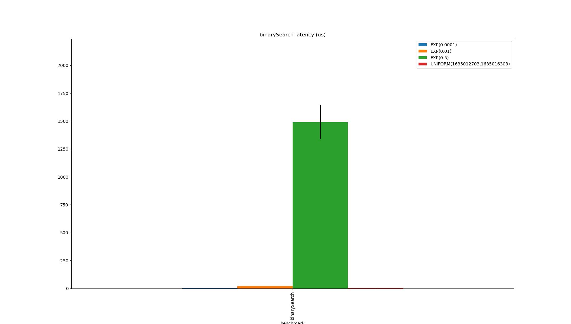
As a baseline, imagine you’re lucky enough to have sorted data and can perform an out-of-the-box binary search.
Arrays.binarySearch doesn’t make guarantees about which index is produced when there are duplicates so a linear scan is needed to find it after yielding an index (though this could use, say, a quadratic probing algorithm).
public class BinarySearch implements RangeEvaluator {

  private final long[] data;

  public BinarySearch(long[] data) {
    this.data = data;
  }

  @Override
  public RoaringBitmap between(long min, long max) {
    int start = Arrays.binarySearch(data, min);
    int begin = start >= 0 ? start : -start - 1;
    while (begin - 1 >= 0 && data[begin - 1] == min) {
      begin--;
    }
    int end = Arrays.binarySearch(data, begin, data.length, max);
    int finish = end >= 0 ? end : -end - 1;
    while (finish + 1 < data.length && data[finish + 1] == max) {
      finish++;
    }
    return RoaringBitmap.bitmapOfRange(begin, finish + 1);
  }

  @Override
  public int serializedSize() {
    return 0;
  }

}
Whilst this has no spatial overhead, the linear search is problematic and it can perform quite badly when there are many duplicates (see $\exp(0.5)$).
To get around this, the data structure below is a naive approximation to Apache Pinot’s sorted index:
public class IntervalsEvaluator implements RangeEvaluator {

  private final long[] uniqueValues;
  private final int[] ranges;

  public IntervalsEvaluator(long[] values) {
    long[] unique = new long[16];
    int[] ranges = new int[16];
    int numRanges = 0;
    int start = 0;
    long current = values[0];
    for (int i = 1; i < values.length; i++) {
      long value = values[i];
      if (current != value) {
        if (numRanges == unique.length) {
          unique = Arrays.copyOf(unique, numRanges * 2);
          ranges = Arrays.copyOf(ranges, numRanges * 2);
        }
        unique[numRanges] = current;
        ranges[numRanges] = start;
        numRanges++;
        current = value;
        start = i;
      }
    }
    unique[numRanges] = current;
    ranges[numRanges] = start;
    numRanges++;
    this.uniqueValues = Arrays.copyOf(unique, numRanges);
    this.ranges = Arrays.copyOf(ranges, numRanges);
  }

  @Override
  public RoaringBitmap between(long min, long max) {
    int start = Arrays.binarySearch(uniqueValues, min);
    int begin = start >= 0 ? start : -start - 1;
    int end = Arrays.binarySearch(uniqueValues, begin, uniqueValues.length, max + 1);
    int finish = end >= 0 ? end : -end - 1;
    return RoaringBitmap.bitmapOfRange(ranges[start], ranges[finish]);
  }

  @Override
  public int serializedSize() {
    return uniqueValues.length * Long.BYTES + ranges.length * Integer.BYTES;
  }
}
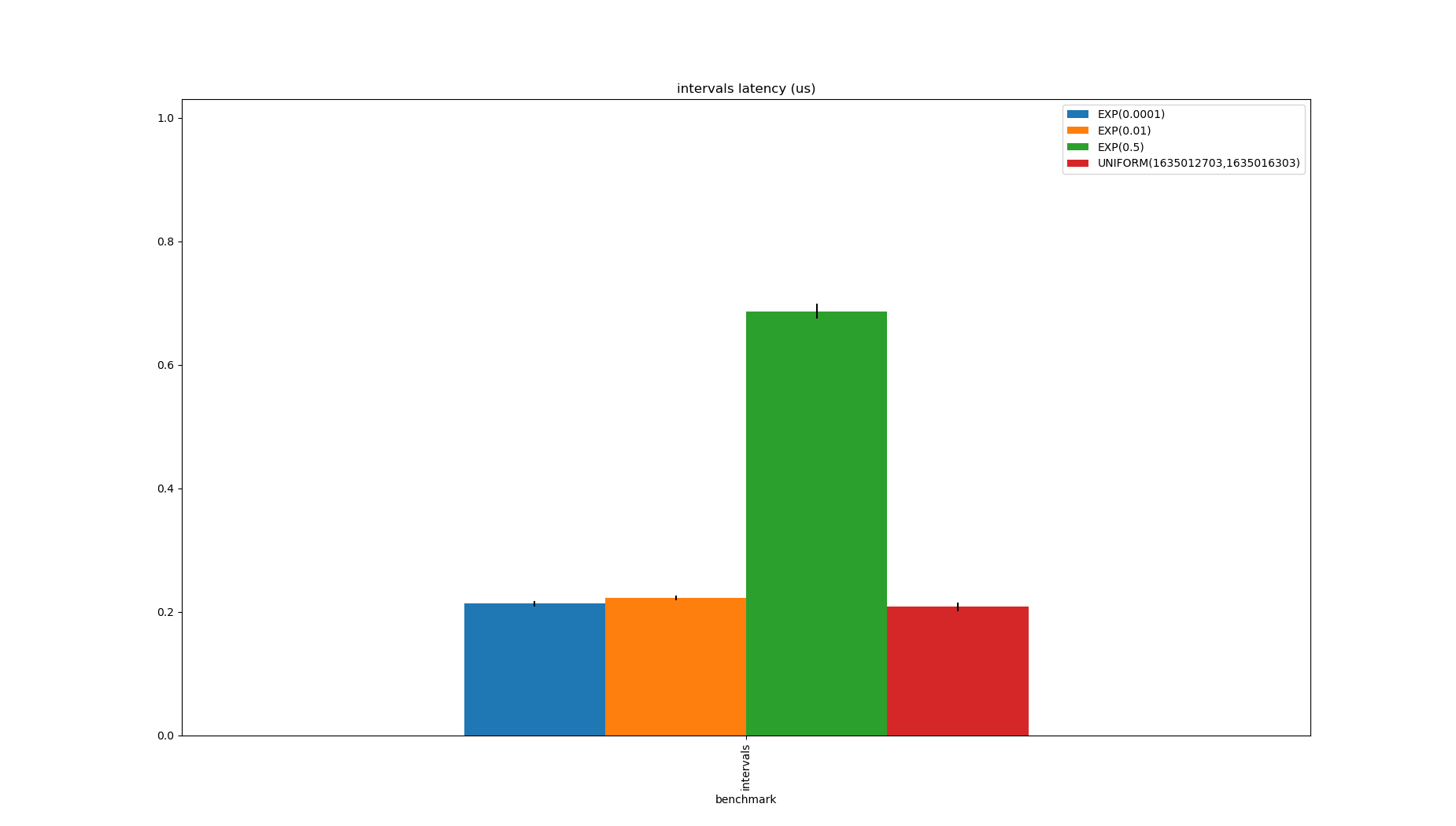
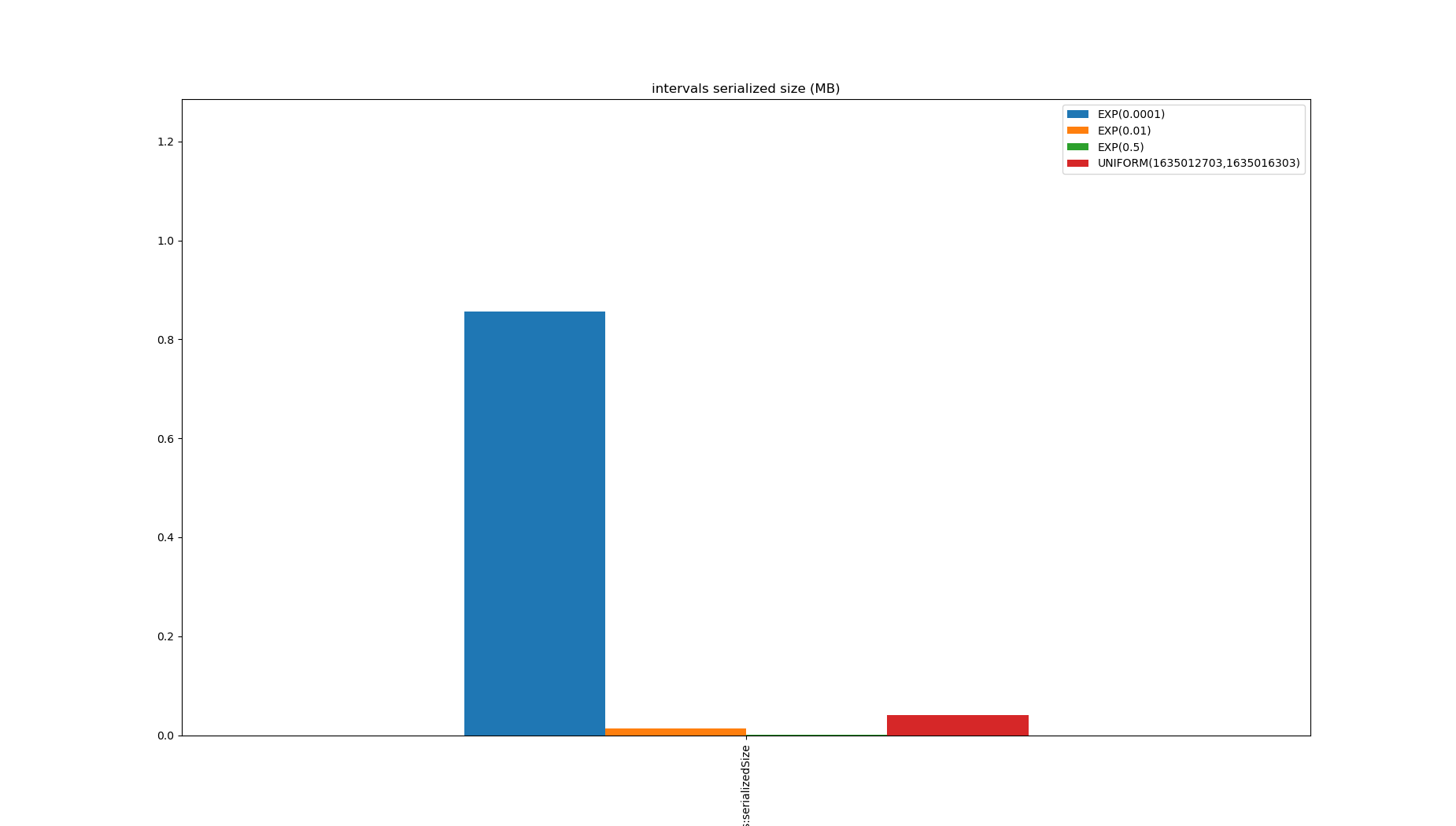
This could be micro-optimised for locality, but it’s hard to beat for this problem, even though it has a spatial overhead of up to 1.5x the size of the input.
Note that the $\exp(0.5)$ case is slower because the range is larger because there are lots of duplicates, but none of these distributions produce unique values, so the size is always smaller than the data.
 In fact, none of the approaches which support range queries over unsorted data will even get close to this.
The first implementation to support unsorted inputs is a natural extension of binary search: make a copy of the data, sort it, and store an array of the indexes where the value was stored in the unsorted array. This is included as a proxy for the way trees which sort the values but not the indexes which I never found justification to implement. These would also need to store and post-process the indexes.
public class SortedValuesUnsortedIndexesEvaluator implements RangeEvaluator {

  private final long[] sortedValues;
  private final int[] indexes;

  public SortedValuesUnsortedIndexesEvaluator(long[] data) {
    List<LongIntPair> pairs = IntStream.range(0, data.length)
        .mapToObj(i -> new LongIntPair(data[i], i))
        .sorted()
        .collect(Collectors.toList());
    sortedValues = pairs.stream().mapToLong(pair -> pair.value).toArray();
    indexes = pairs.stream().mapToInt(pair -> pair.index).toArray();
  }

  @Override
  public RoaringBitmap between(long min, long max) {
    int start = Arrays.binarySearch(sortedValues, min);
    int begin = start >= 0 ? start : -start - 1;
    while (begin - 1 >= 0 && sortedValues[begin - 1] == min) {
      begin--;
    }
    int end = Arrays.binarySearch(sortedValues, begin, sortedValues.length, max);
    int finish = end >= 0 ? end : -end - 1;
    while (finish + 1 < sortedValues.length && sortedValues[finish + 1] == max) {
      finish++;
    }
    RoaringBitmap result = new RoaringBitmap();
    for (int i = begin; i < finish; i++) {
      result.add(indexes[i]);
    }
    return result;
  }

  @Override
  public int serializedSize() {
    return sortedValues.length * Long.BYTES + indexes.length * Integer.BYTES;
  }

  private static final class LongIntPair implements Comparable<LongIntPair> {

    private final long value;
    private final int index;

    private LongIntPair(long value, int index) {
      this.value = value;
      this.index = index;
    }

    @Override
    public int compareTo(LongIntPair o) {
      return Long.compare(value, o.value);
    }

    @Override
    public boolean equals(Object o) {
      if (this == o) {
        return true;
      }
      if (o == null || getClass() != o.getClass()) {
        return false;
      }

      LongIntPair that = (LongIntPair) o;

      if (value != that.value) {
        return false;
      }
      return index == that.index;
    }

    @Override
    public int hashCode() {
      int result = (int) (value ^ (value >>> 32));
      result = 31 * result + index;
      return result;
    }
  }
}
This doesn’t perform very well, and storing it requires 1.5x the size of the data, despite finding the boundaries quickly when there are few duplicates.
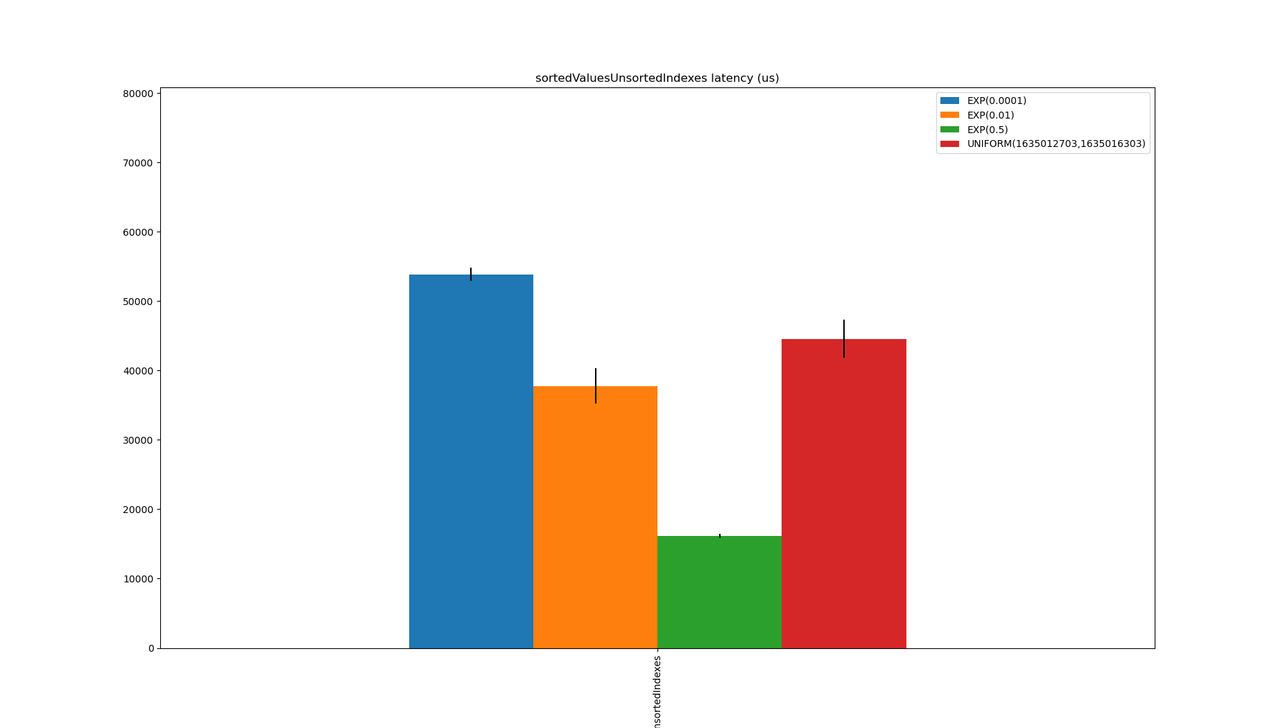
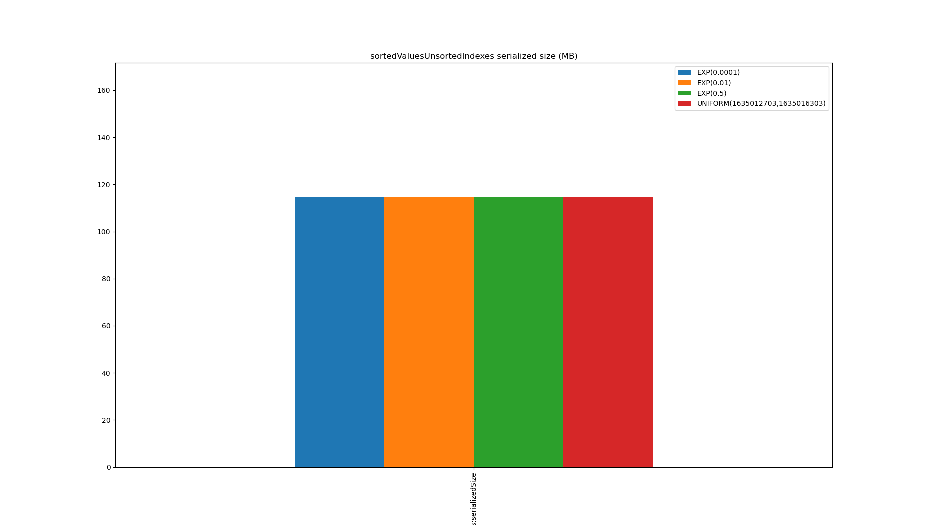
Part of the problem is it’s not very efficient to build a RoaringBitmap from unsorted data, and maybe Pinot needing a RoaringBitmap is an artificial constraint.
If building a RoaringBitmap weren’t the bottleneck, copying and sorting a section of the indexes array might be.
InvertedIndexEvaluator is a natural extension of IntervalsEvaluator, instead of storing the start of the range, it stores a bitmap of row indexes which have the value.
public class InvertedIndexEvaluator implements RangeEvaluator {

  private final long[] uniqueValues;
  private final RoaringBitmap[] bitmaps;
  private final int serializedSize;

  public InvertedIndexEvaluator(long[] values, long[] sortedValues) {
    long[] unique = new long[16];
    int numRanges = 0;
    long current = sortedValues[0];
    for (int i = 1; i < sortedValues.length; i++) {
      long value = sortedValues[i];
      if (current != value) {
        if (numRanges == unique.length) {
          unique = Arrays.copyOf(unique, numRanges * 2);
        }
        unique[numRanges] = current;
        numRanges++;
        current = value;
      }
    }
    unique[numRanges] = current;
    numRanges++;
    this.uniqueValues = Arrays.copyOf(unique, numRanges);
    RoaringBitmapWriter<RoaringBitmap>[] writers = new RoaringBitmapWriter[numRanges];
    Arrays.setAll(writers, i -> RoaringBitmapWriter.writer().get());
    for (int i = 0; i < values.length; i++) {
      writers[Arrays.binarySearch(uniqueValues, values[i])].add(i);
    }
    RoaringBitmap[] bitmaps = new RoaringBitmap[writers.length];
    Arrays.setAll(bitmaps, i -> writers[i].get());
    this.bitmaps = bitmaps;
    int ss = uniqueValues.length * 8 + bitmaps.length * 4;
    for (RoaringBitmap bitmap : bitmaps) {
      ss += bitmap.serializedSizeInBytes();
    }
    this.serializedSize = ss;
  }

  @Override
  public RoaringBitmap between(long min, long max) {
    int start = Arrays.binarySearch(uniqueValues, min);
    int begin = start >= 0 ? start : -start - 1;
    int end = Arrays.binarySearch(uniqueValues, begin, uniqueValues.length, max + 1);
    int finish = end >= 0 ? end : -end - 1;
    RoaringBitmap bitmap = bitmaps[begin].clone();
    for (int i = begin + 1; i <= finish & i < bitmaps.length; i++) {
      bitmap.or(bitmaps[i]);
    }
    return bitmap;
  }

  @Override
  public int serializedSize() {
    return serializedSize;
  }
}
This is a good option when there are a lot of duplicates, but needing to merge many tiny bitmaps to produce an output is the bottleneck.
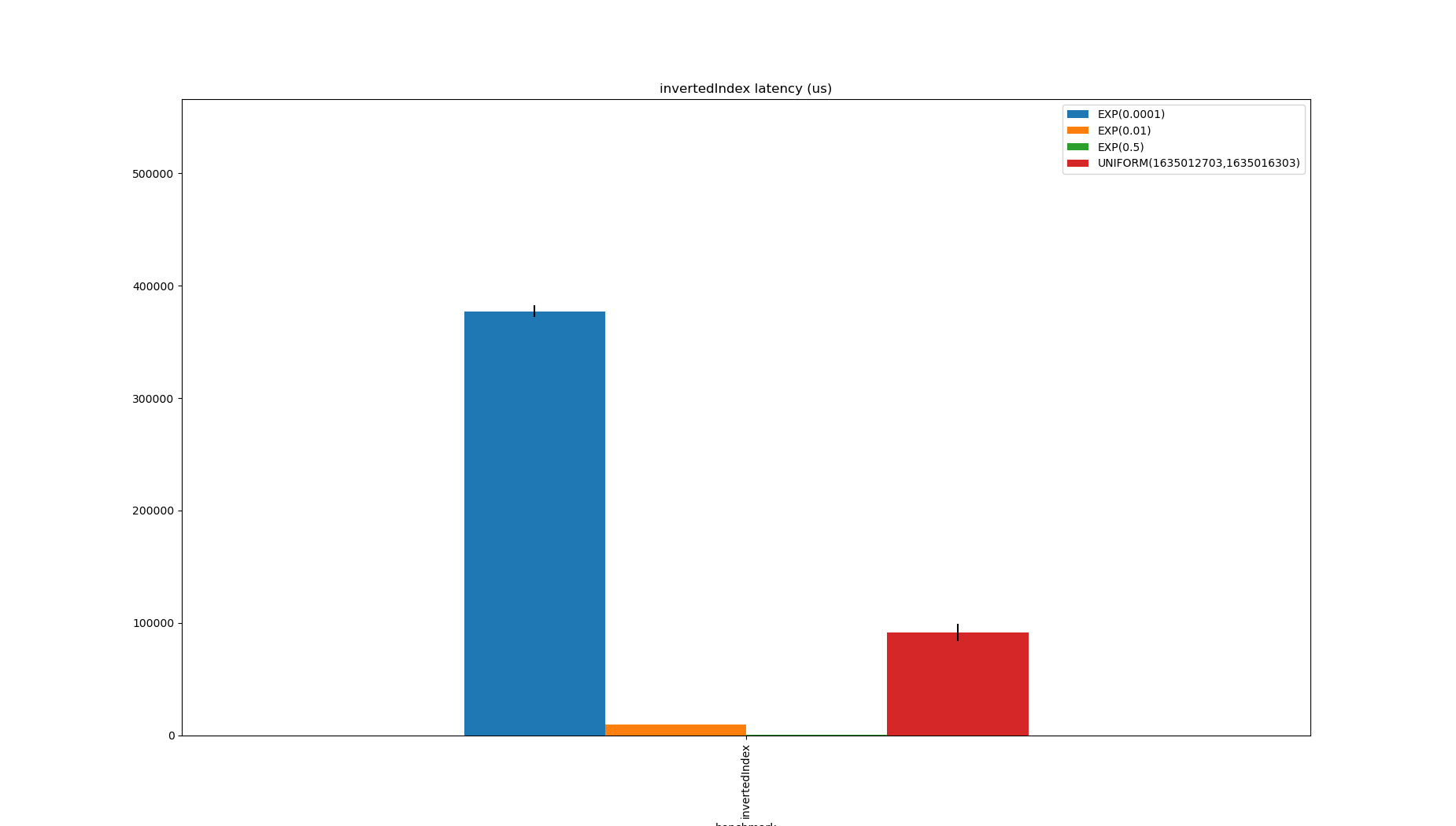
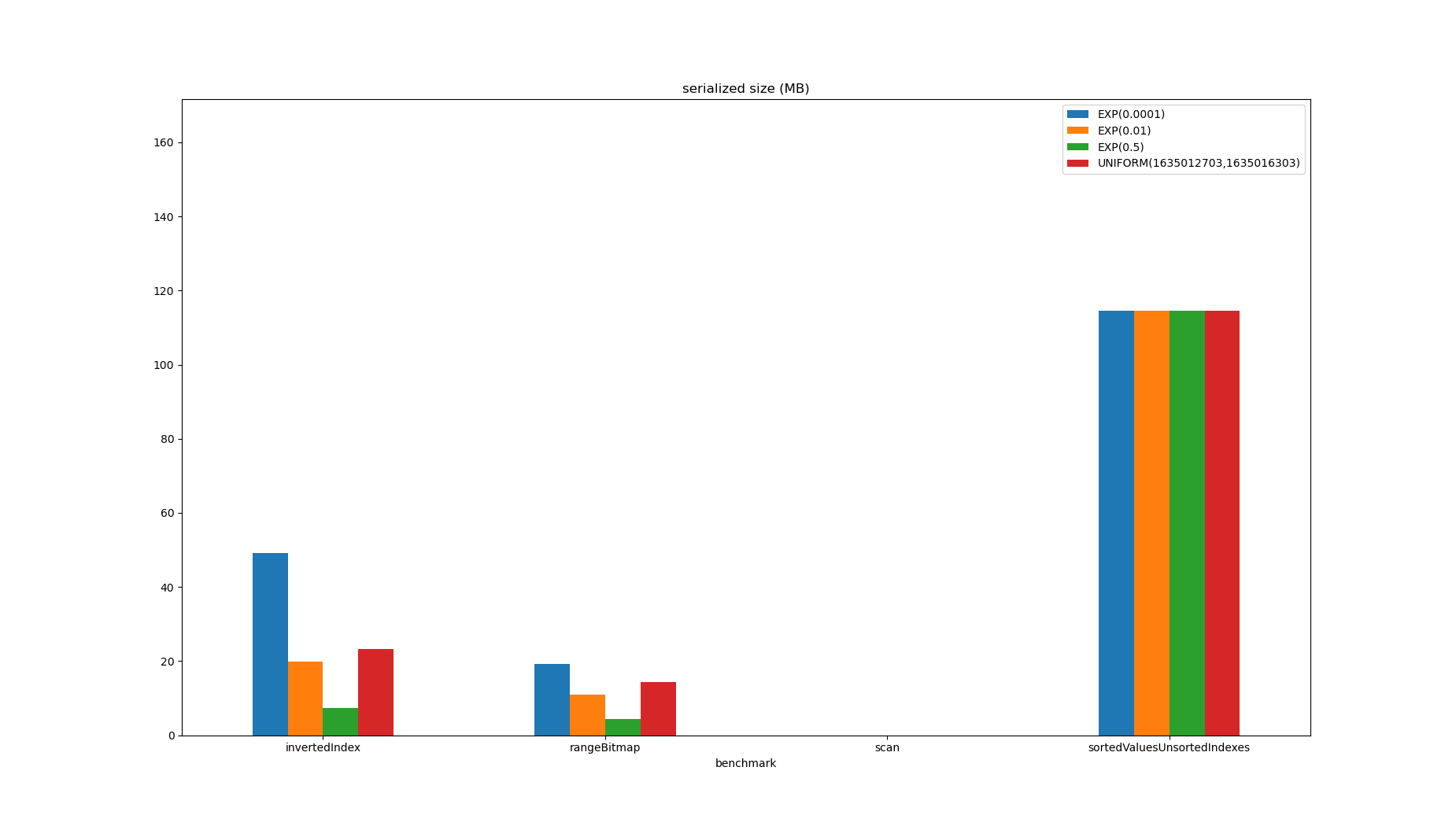
The index is always smaller than the data:
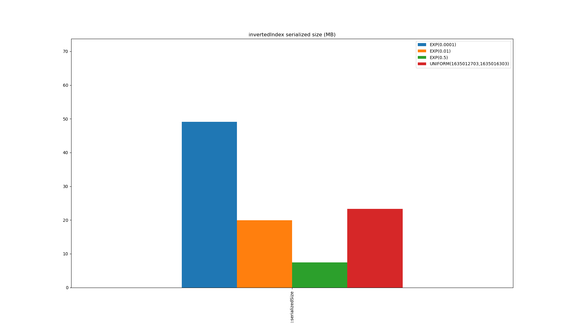
Pinot’s old range index was quite similar to this, except the posting lists corresponded to buckets, and required a scan to remove false positives after filtering. By range encoding an inverted index (that is, when indexing a row with a value update all posting lists greater than the value too) range queries can be very fast, but the indexes end up huge and the consequent write amplification is unacceptable.
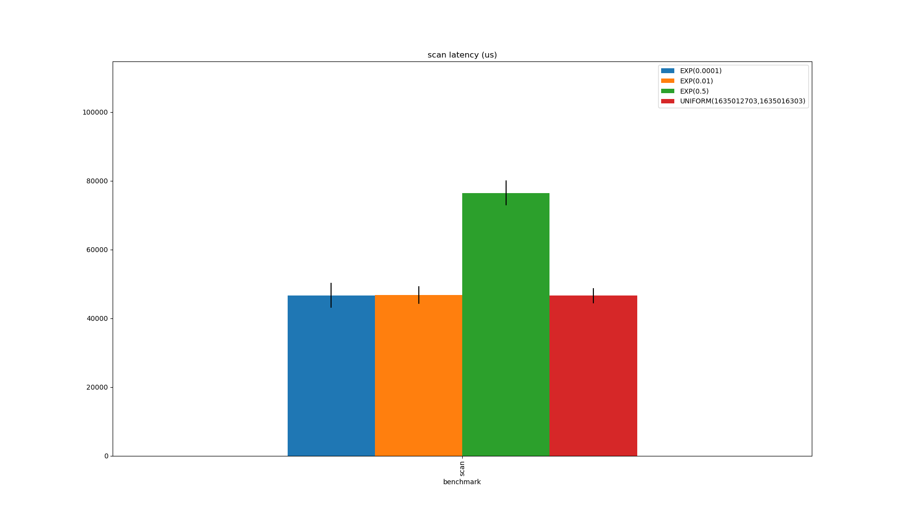
The simplest approach is a scan:
public class Scan implements RangeEvaluator {

  private final long[] data;

  public Scan(long[] data) {
    this.data = data;
  }

  @Override
  public RoaringBitmap between(long min, long max) {
    RoaringBitmapWriter<RoaringBitmap> writer = RoaringBitmapWriter.writer().get();
    for (int i = 0; i < data.length; i++) {
      if (data[i] >= min && data[i] <= max) {
        writer.add(i);
      }
    }
    return writer.get();
  }

  @Override
  public int serializedSize() {
    return 0;
  }
}
This has no spatial overhead but is very slow, though this could be done a lot faster by Java programs once the Vector API is available so will be a better option in the future.
Finally, RangeBitmap:
public class RangeBitmapEvaluator implements RangeEvaluator {

  private final RangeBitmap bitmap;
  private final int serializedSize;

  public RangeBitmapEvaluator(long[] data) {
    long min = Long.MAX_VALUE;
    long max = Long.MIN_VALUE;
    for (long datum : data) {
      min = Math.min(min, datum);
      max = Math.max(max, datum);
    }
    var appender = RangeBitmap.appender(max);
    for (long datum : data) {
      appender.add(datum - min);
    }
    serializedSize = appender.serializedSizeInBytes();
    this.bitmap = appender.build();
  }

  @Override
  public RoaringBitmap between(long min, long max) {
    return bitmap.between(min, max);
  }

  @Override
  public int serializedSize() {
    return serializedSize;
  }
}
It doesn’t get close to IntervalsEvaluator, but it’s the least bad considered option for unsorted values, it is always smaller than the data.
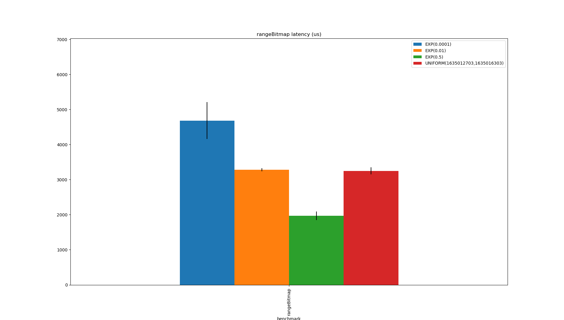
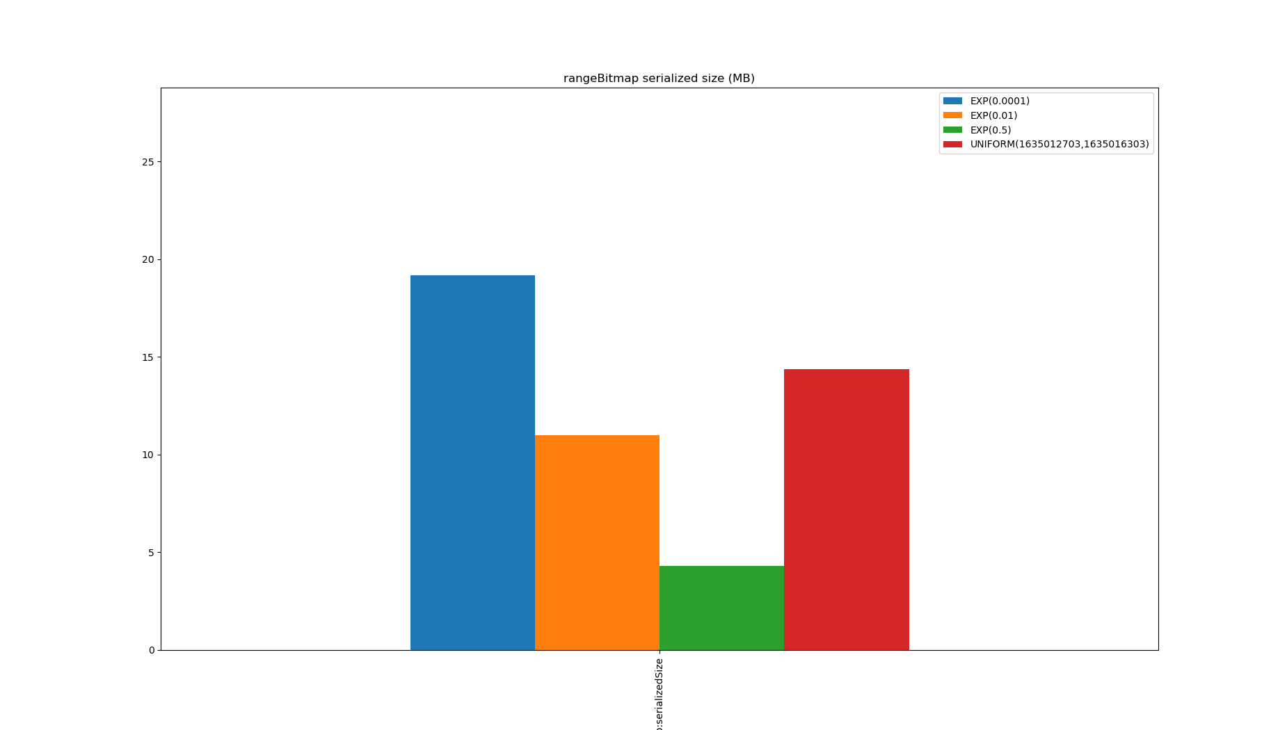
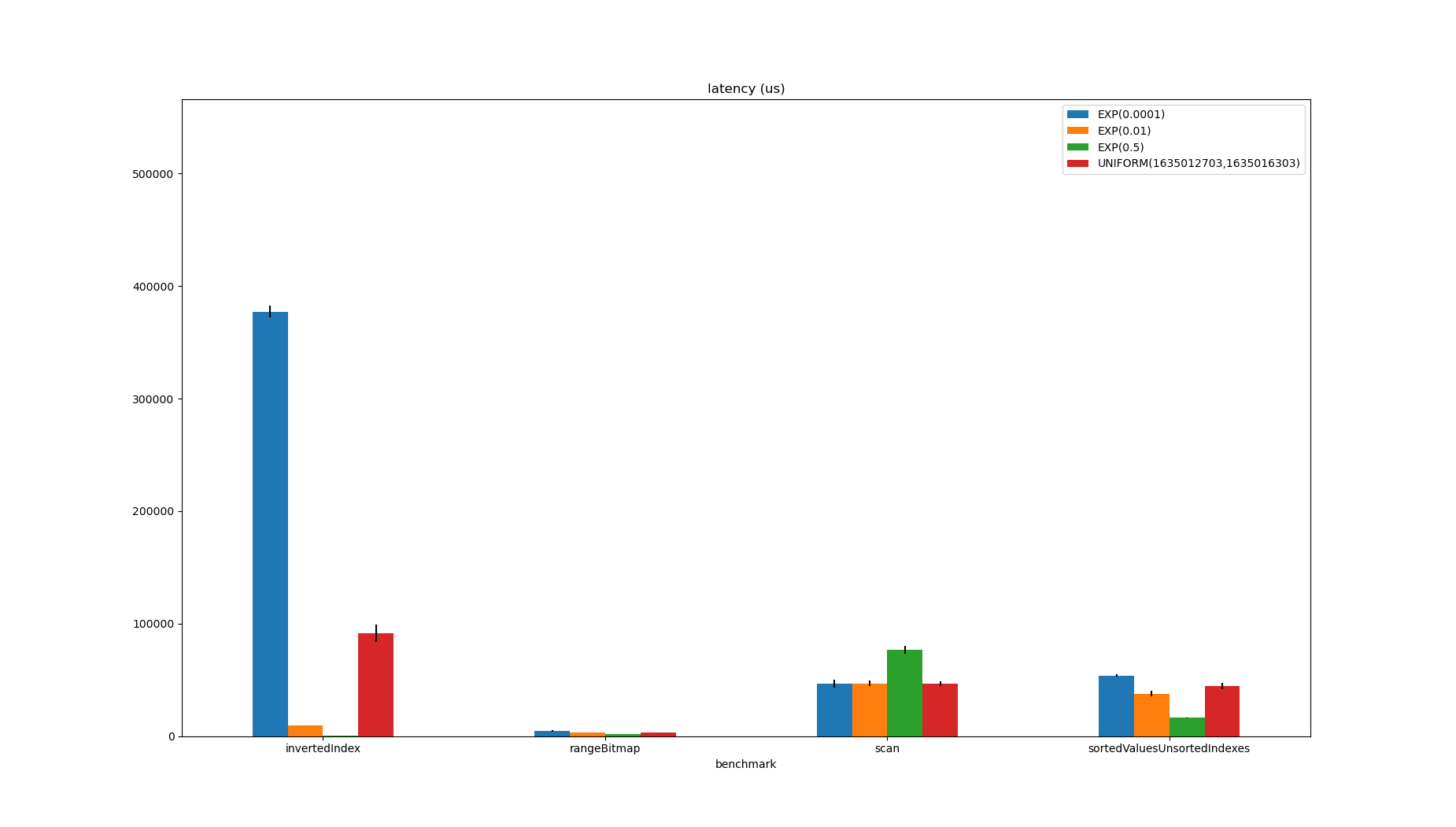
Excluding the implementations which only work on sorted inputs, RangeBitmap looks like the least bad option.
It is only beaten by the inverted index in one case, is an order of magnitude faster than scanning or the sorted-values/unsorted-indexes approach and the inverted index in other cases.
It also has the least spatial overhead except for scanning which has none.
The source code for these benchmarks is located here
Usage in Apache Pinot
Apache Pinot allows range indexing of immutable segments, and since 0.9.0 these have been implemented in terms of RangeBitmap, enabled via a feature flag.
From 0.10.0, this feature flag is enabled by default, and just needs the configuration in the documentation here.
Users who have enabled the feature flag (which I won’t name: just upgrade to 0.10.0) have reported improvements of upwards of 5x on Pinot’s old range index implementation.
Links:
- StarTree blog covers Apache Pinot
- StarTree YouTube channel curates Apache Pinot related content
- Apache Pinot Slack channel
- Apache Pinot project on github
- Apache Pinot documentation
- Apache Pinot Range index design document
- Apache Pinot range index creator and reader
- RoaringBitmap Java Library
RangeBitmapimplementation- High level overview of Pinot range queries