Population Dynamics Part 1: Population Level Models
This post is the first in a series about the counter-intuitive dynamics of a predator-prey ecosystem in dynamic equilibrium, which was the topic of my undergraduate dissertation, based on the paper Predator-prey cycles from resonant amplification of demographic stochasticity. It seems strange to dig this up over a decade later, but thanks to COVID-19, the sibling field of epidemiology is now a casual topic of conversation, which got me thinking back to this project. The project made a lasting impression on me because the model’s ergodic assumption - that time and ensemble averages are interchangeable - is violated both by data and by numerical simulation. The average behaviour predicted by the model is never realised, and observed dynamics can only be explained by looking at higher order terms of the so-called noise expansion.
The aim of modeling population dynamics is to understand how population levels change over time. Once you have a model, you can use it to do numerical experiments to predict how an environmental policy will impact populations, in order to avoid, say, inadvertently making a species go extinct. When research into population dynamics began, some of the tools we have now, such as computers and stochastic calculus, did not exist, but differential equations were well understood. The classical approach is known as population level modeling, which involves writing down coupled differential equations for the population (actually, the density is modeled, see below) of each species, as a function of time. Each interspecies interaction (e.g. lions eating zebras) is represented as a parameter, which can be inferred from data (i.e. you can actually observe how many zebras are hunted per lion per unit of time).
I’m not qualified to comment on the practical use of these models, but they make some mathematical assumptions which seem strange:
- Populations must be differentiable, which implies continuity, whereas birth/death events are discrete (it’s impossible to kill or give birth to a fractional zebra).
- It follows that populations must be infinite.
For these reasons, it can sort of make sense if population density, defined as the ratio of a species population to all populations, is modeled instead of population. The differential equations describe what happens when the populations become infinite, and the models are more appropriate the larger the population sizes.
Lotka-Volterra Model
The Lotka-Volterra model is a very old and simple example of a two species population level model. The prey reproduce at a rate proportional to their population density and have infinite resources; natural death does not occur. The predators only eat the prey, and also reproduce at a rate proportional to their population density.
Suppose there are $M$ prey and $N$ predators, we have population densities $m=\frac{M}{M+N}$ and $n = \frac{N}{M+N}$ which take values in $[0, 1]$ if the system doesn’t grow. The model is simply:
\[\begin{aligned} \frac{dm}{dt} &= am - bmn\\ \frac{dn}{dt} &= cmn - dn \end{aligned}\]Here,
- $a$ is the non-negative prey growth rate.
- $b$ is the non-negative predation rate.
- $c$ is the non-negative birth rate of the predators (linked to predation).
- $d$ is the non-negative predator death rate.
There are three obvious conclusions:
- If the predators go extinct, the prey grow exponentially ($\frac{dm}{dt} = am \implies m(t) = \exp(at)$).
- If the prey go extinct, the predators will go extinct shortly after ($\frac{dn}{dt} = -dn \implies n(t) = \exp(-dt)$).
- If both species go extinct, nothing changes.
To get more out of the model, such as answering questions like
- Can either species go extinct?
- Can the population levels oscillate?
- Do they oscillate in phase or out of phase?
- Do the population levels stabilise?
Some maths is required, but we don’t actually have to solve the equations!
Stability Analysis
The system of equations is a nonlinear dynamical system, and there is a lot of theory to help with performing a qualitative analysis. To understand the dynamics, imagine standing at a point $(m_t, n_t)$ in a 2D space, you are facing the direction $(\frac{dm}{dt}, \frac{dn}{dt})$. As you move in this direction, the direction keeps changing according to the system’s dynamics, and you trace a path or a trajectory in space. If you started somewhere else, at $(m’_t, n’_t)$, you would take a different path. To reason about system stability, we need to know about these paths and how they relate to each other. For instance:
- Are there paths which lead to the same point?
- Are there points which can never be left?
- Is it possible to go round in circles?
- Are there paths which never stop?
The basic idea is to find the fixed points of the system, and then analyse a linear approximation of the system very close to these fixed points.
Fixed Points
By “find the fixed points of the system” I mean find the values of $(m, n)$ where the equations are equal to zero. By inspection, there is a trivial fixed point at $\mathbf{0}$. Setting the equations to zero, we get expression where $m$ and $n$ are constant, and just need to intersect them to find fixed points.
\[\begin{aligned} \frac{dm}{dt} &= am - bmn = 0\\ \frac{dn}{dt} &= cmn - dn = 0 \\ \implies n &= \frac{a}{b}\\ m &= \frac{d}{c} \\ \end{aligned}\]So, $(d/c, a/b)$ is a more interesting fixed point of this system.
Linearisation
By “analyse a linear approximation” I mean pretend the system is actually of the form below, where the coefficient names are coincidental:
\[\begin{aligned} \frac{dm}{dt} &= am + bn \\ \frac{dn}{dt} &= cm + dn \\ \text{ let } A &= \left(\begin{array}{cc} a & b\\ c & d \end{array}\right) \text{, } \mathbf{x}=\left(\begin{array}{}m \\ n\end{array}\right)\\ \frac{d\mathbf{x}}{dt} &= A \mathbf{x} \end{aligned}\]The only fixed point in this system is $\mathbf{0}$; if we start there, we can’t leave, but every other point leads to another. We can understand what happens elsewhere than $\mathbf{0}$ by looking at the eigenvalues of the matrix, which we get from the roots of the characteristic polynomial (see the Cayley-Hamilton theorem).
\[\begin{aligned} P(\lambda) &= |A - \lambda I| \\ &= \left|\left(\begin{array}{cc} a - \lambda & b\\ c & d - \lambda \end{array}\right)\right| \\ &= \lambda^2 - 2(a + d)\lambda + ad - bc\\ \Delta = |A| &= ad - bc\\ \tau = \mathbf{Trace}(A) &= a + d \\ \implies P(\lambda) &= \lambda^2 - 2\tau + \Delta \end{aligned}\]The solutions of this quadratic equation are the system’s eigenvalues. If we know the eigenvalues, we can find the Jordan form $M^{-1}AM$ of the matrix $A$, which determines the stability type.
If $\tau^2 - \Delta > 0$, the eigenvalues $\lambda_1, \lambda_2$ are distinct and real-valued. There exists a matrix $M$ such that:
\[M^{-1}AM = \left(\begin{array}{cc} \lambda_1 & 0\\ 0 & \lambda_2 \end{array}\right) \\\]The dynamics then depends on the signs of the eigenvalues. If they are both negative, the system has a stable node; if they are both positive, an unstable node; if they are of opposite sign, a saddle: stable in one direction (eigenvector), unstable in the other.
If $\tau^2 - \Delta < 0$, the eigenvalues $\lambda_1, \lambda_2$ are distinct and complex-valued; the stability types are discriminated by the sign of the real component of the eigenvalues. There exists a matrix $M$ such that:
\[M^{-1}AM = \left(\begin{array}{cc} u & -v\\ v & u \end{array}\right) \\\]If the real component of the eigenvalue is negative, the system is stable; if positive, the system is unstable; if zero the system has cycles.
This means the different stability types a linear system can exhibit can be plotted as contiguous regions of $(\tau, \Delta)$ space.
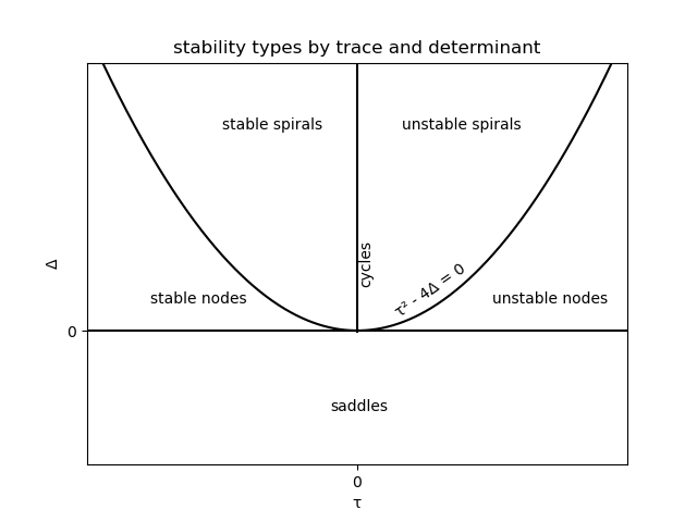
All of this is only strictly true for linear systems, but we want to analyse nonlinear systems. Thanks to the Hartman-Grobman theorem, a nonlinear system can be approximated by a linear system $\frac{dm}{dt} = f(m, n), \frac{dn}{dt} = g(m, n)$ within a neighbourhood of a fixed point without changing the stability type, so long as the fixed point is hyperbolic.
The Poincaré–Bendixson theorem shows that only the outlined stability types and limit cycles are possible in 2D models; they are too simple to be chaotic. To characterise a 2D nonlinear system, make a linear approximation, and then just calculate the trace and determinant which implies the stability type.
So, if $(m’, n’)$ is a fixed point, the linear approximation can be derived by considering points $(u, v) = (m-m’, n-n’)$ and performing a Taylor expansion about $(m’, n’)$, we get a linear system, obtaining the Jacobian matrix at the fixed point.
\[\begin{aligned} \left(\begin{array}{c}\frac{du}{dt} \\ \frac{dv}{dt} \end{array}\right) &= \left(\begin{array}{c}f(m' + u, n' + v) \\ g(m' + u, n' + v) \end{array}\right) \\ &= \left(\begin{array}{c}f + u\frac{\partial f}{\partial m} + v\frac{\partial f}{\partial n} + \mathcal{O}(u^2, v^2, uv) \\ g + u\frac{\partial g}{\partial m} + v\frac{\partial g}{\partial n} + \mathcal{O}(u^2, v^2, uv) \end{array}\right)_{(m', n')} \\ &\approx \left(\begin{array}{c}u\frac{\partial f}{\partial m} + v\frac{\partial f}{\partial n} \\ u\frac{\partial g}{\partial m} + v\frac{\partial g}{\partial n} \end{array}\right)_{(m', n')} \\ &= \left(\begin{array}{cc}\frac{\partial f}{\partial m} & \frac{\partial f}{\partial n} \\ \frac{\partial g}{\partial m} & \frac{\partial g}{\partial n} \end{array}\right)_{(m', n')}\left(\begin{array}{c}u \\ v \end{array}\right) \end{aligned}\]In the steps above, the terms of quadratic order are allowed to disappear because of the Hartman-Grobman theorem, but it should be checked that the fixed point is hyperbolic. This matrix and its eigenvalues help to find the stability type of the system.
Lotka-Volterra Stability Analysis
To figure out whether the species go extinct, grow exponentially, stabilise, or cycle, just three steps are required.
- Find the fixed points.
- Compute the Jacobian matrix at the fixed points.
- Calculate the trace and determinant of the Jacobian at each fixed point and look up the stability type.
The nontrivial fixed point at $(d/c, a/b)$ was already calculated above; now the Jacobian.
\[\begin{aligned} \mathcal{J}(m', n') &=\left(\begin{array}{cc}\frac{\partial}{\partial m}(am - bmn) & \frac{\partial }{\partial n} (am - bmn) \\ \frac{\partial }{\partial m} (cmn - dn) & \frac{\partial }{\partial n} (cmn - dn) \end{array}\right)_{(m', n')} \\ &= \left(\begin{array}{cc}a - bn & -bm \\ cn & cm - d \end{array}\right)_{(m', n')}\\ &= \left(\begin{array}{cc}0 & -bd/c \\ ca/b & 0 \end{array}\right)\\ \end{aligned}\]The trace is zero, and the determinant is $ad$, which is positive, so the model predicts cycles around to this point.
Now the extinction fixed point $\mathbf{0}$.
\[\begin{aligned} \mathcal{J}(0, 0) &= \left(\begin{array}{cc}a - bn & -bm \\ cn & cm - d \end{array}\right)_{(0, 0)}\\ &= \left(\begin{array}{cc}a & 0 \\ 0 & -d \end{array}\right)\\ \end{aligned}\]The trace is $a-d$, but the determinant $-ad$, which is always negative, so the fixed point is a saddle (convergent in one approach, divergent in another).
This can be visualised with a bit of python.
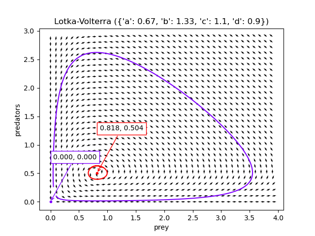
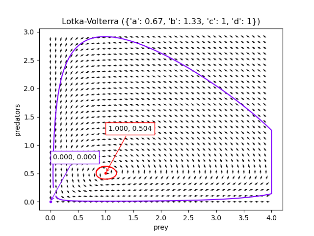
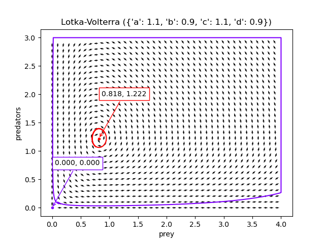
If the population densities start off close to $(d/c, a/b)$ (the red dot), there are tight oscillations. If the population densities start off close to $\mathbf{0}$ (the purple dot), there are larger oscillations, but the species won’t actually go extinct.
The code to generate these visualisations is at Github, but I found a scipy tutorial for creating these charts in a much better way afterwards, presumably written by a competent python programmer.
Volterra Model
The cycles in the Lotka-Volterra model correspond reasonably well to patterns observed in nature, but the assumption in the Lotka-Volterra model that prey populations grow exponentially in the absence of predation is unrealistic. Finite resources means growth should be sigmoidal, and this is especially important in harsh environments like tundra. The model can be modified to include a carrying capacity to ensure bounded prey growth, Modelling Biological Populations in Space and Time calls this model the Volterra model.
The model is simply:
\[\begin{aligned} \frac{dm}{dt} &= m(a - bm - cn)\\ \frac{dn}{dt} &= n(em - d) \end{aligned}\]Where,
- $a$ is the non-negative prey growth rate.
- $b$ is the non-negative carrying capacity.
- $c$ is the non-negative predation rate.
- $d$ is the non-negative birth rate of the predators (linked to predation).
- $e$ is the non-negative predator death rate.
Again, the equations don’t need to be solved to understand how the system evolves; evaluating the Jacobian matrix at each fixed point is enough. Trivially, there is a fixed point at $\mathbf{0}$; if the prey go extinct, so will the predators. If the predators go extinct ($n=0$), then the prey will converge to the carrying capacity. The fixed point is $(a/b, 0)$.
\[\begin{aligned} \frac{dm}{dt} &= m(a - bm) = 0\\ \implies m &= \frac{a}{b} \end{aligned}\]There is another fixed point where $\frac{dm}{dt}$ and $\frac{dn}{dt}$ intersect.
\[\begin{aligned} \frac{dm}{dt} &= m(a - bm - cn) = 0\\ \frac{dn}{dt} &= n(em - d) = 0\\ &\implies \begin{cases} m \text{ stationary on }n = \frac{a -bm}{c}\\ n \text{ stationary on }m = \frac{d}{e}\\ \end{cases}\\ &\implies (\frac{d}{e}, \frac{a-\frac{bd}{e}}{c}) \text{ is fixed } \end{aligned}\]The Jacobian, to be evaluated at each fixed point, is:
\[\begin{aligned} \mathcal{J}(m', n') &=\left(\begin{array}{cc}\frac{\partial}{\partial m}m(a - bm - cn) & \frac{\partial }{\partial n} m(a - bm - cn) \\ \frac{\partial }{\partial m} n(em - d) & \frac{\partial }{\partial n} n(em - d) \end{array}\right)_{(m', n')} \\ &= \left(\begin{array}{cc}a - 2bm - cn & -cm \\ ne & em - d \end{array}\right)_{(m', n')} \end{aligned}\]At $\mathbf{0}$ (mutual extinction) the trace is $a - d$, and determinant $ad$: it’s still a saddle. At $(a/b, 0)$ (predator extinction) the trace is $a(e/b - 1) - d$, and the determinant is $a (d - ea/b)$. Each of these expressions can be positive or negative; the point’s stability type depends on the values of the parameters. At the nontrivial fixed point, we have
\[\begin{aligned} \mathcal{J} &= \left(\begin{array}{cc}-b\frac{d}{e} & -c\frac{d}{e} \\ \frac{ae-bd}{c} & 0 \end{array}\right)\\ \implies \tau &= -b\frac{d}{e}\\ \Delta &= d\left(\frac{bd}{e}-a\right)\\ \end{aligned}\]Whenever $a < bd/e$, the determinant is positive, but the trace is always negative, so the model predicts convergence.
Actually, there could still be a limit cycle in the system, but it can be ruled out using Dulac’s criterion. If there exists a function $h$ such that $\mathrm{div}(h \cdot (\frac{dm}{dt}\mathbf{m} + \frac{dn}{dt}\mathbf{n}))$ does not change sign in some region of phase space, there are no cycles in that region. Since this is a population model, only the positive quadrant is important, so, choosing $h = 1/mn$:
\[\begin{aligned} \mathrm{div}(h \cdot (\frac{dm}{dt}\mathbf{m} + \frac{dn}{dt}\mathbf{n})) &= \frac{\partial}{\partial m}h\frac{dm}{dt} + \frac{\partial}{\partial n}h\frac{dn}{dt}\\ &= \frac{\partial}{\partial m}\frac{a-bm-cn}{n} + \frac{\partial}{\partial n} \frac{em-d}{m}\\ &= -\frac{b}{n} \end{aligned}\]$-\frac{b}{n}$ doesn’t change sign when $n$ is positive, so the system can’t have any limit cycles, so is convergent.
This can be shown by visualisation, configured with reasonable parameters for a harsh tundra environment. With almost all initial conditions, the system converges to $(\frac{d}{e}, \frac{a-\frac{bd}{e}}{c})$ (the red dot).
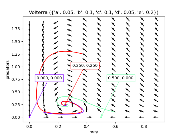
This is all very well, but many ecosystems do oscillate, even those in harsh environments, and no calibration can make this system oscillate. Making the realistic assumption that there is a carrying capacity - or natural death among prey - prevents the model from predicting real population dynamics.
Wrap Up
I covered two models based on coupled differential equations, one with unrealistic ecological assumptions but good predictions, the other with realistic assumptions but unrealistic predictions. Ultimately, this is because these models need infinite populations to work, but have been applied to sparse populations where there are thousands or even hundreds of individuals. In the next post, I will cover building the Volterra model up from stochastic individual level dynamics, and show how to derive a master equation for a stochastic dynamical system.
This post involved some qualitative analysis of dynamical systems, if you are interested in this, the book Nonlinear Dynamics and Chaos by Steven Strogatz is great for going in to more depth.