Heuristics for Substring Search
My last post was about adapting an existing substring search algorithm to reduce its memory requirement, but ended with a section about a heuristic approach to the problem. Heuristic optimisation can be a blessing and a curse; they may trade better best case performance for worse worst case performance. I benchmarked my implementations with uniformly random data and found that finding the first byte as quickly as possible before switching into a more intensive search was effective. This heuristic bets on the first byte of the search term being rare, allowing lots of data, on average 256 bytes, to be skipped over quickly between each more thorough examination of the data. Looking at the structure of natural language paints a more interesting picture, making this optimisation questionable.
Structure and sparseness in natural language text
English and German
English and German are both West Germanic languages and very similar, understood to have evolved from a common language known as Proto-Germanic. Similarities, pertinent to the structure of byte arrays, include:
- The alphabets are almost identical.
- There are non-loanword cognates in both languages spelt exactly the same way (e.g. Hand).
- Many English words of Germanic origin have undergone sound shifts known as Grimm’s Law (e.g. β -> t in Fuβ -> foot, or pf -> p in Pfanne -> pan) and no other change. If an English text and a German text have the same semantic content, some of the sequences of bytes will be the same.
- Some English words have undergone sound shifts as well as shifts in meaning, but are ultimately cognate to German words (the word town comes from the Old English tūn meaning “fenced enclosure”, whereas the German Zaun, pronounced tsown, means fence). Many of the sequences of bytes found in English words might be found somewhere in a German text even if they are semantically unrelated.
- Some English words are spelt the same way, but have different meaning (gift vs Gift). Despite texts having different semantic content, the same sequence of bytes could be found in each text.
- The development of both languages was influenced by ecclesiastical Latin during the medieval period. These words have the same spelling, up to conjugation, declension, and minor differences in alphabet.
There are stark differences, pertinent to the structure of byte arrays, too:
- German uses some special characters like β in place of ss, and umlauts for raising or fronting vowels. This means that German uses more code points above 127, and has some UTF-8 characters represented by code points above 255.
- German capitalises nouns, whereas English does not. German texts contain more capital letters than English.
- German regular verbs in the past participle start with ge-; weak verbs replace the ending with t (schaffen -> geschaft, strong verbs keep the ending (essen -> gegessen). Almost all English verbs are weak and just have the suffix -ed in the past participle, some with the archaic -t, such as spelt. German text may have more variability in the character before a space.
- German concatenates nouns and adjectives to create compound nouns. German texts should contain fewer spaces than equivalent English texts.
- There are roughly as many words in English of French origin as of Germanic origin, and English also has many words of Norse origin.
In short, German and English are quite similar, but when encoded as byte arrays probably have different characteristics.
Comparison of King James Bible and Luther 1912 Bible
To show the structural similarities and differences between English and German I collected frequency histograms from the King James Bible and the 1912 revision of the Luther Bible, downloaded here. I chose these texts because they are essentially the same book, translated from the same source by Northern European protestants within 100 years of each other. The texts are frequently obviously equivalent in meaning, given some familiarity with each language:
“Chapter 1. In the beginning God created the heaven and the earth. And the earth was without form, and void; and darkness was upon the face of the deep. And the Spirit of God moved upon the face of the waters. And God said, Let there be light: and there was light.”
“1. Am Anfang schuf Gott Himmel und Erde. Und die Erde war wüst und leer, und es war finster auf der Tiefe; und der Geist Gottes schwebte auf dem Wasser. Und Gott sprach: Es werde Licht! und es ward Licht. “
Both texts had major impacts on the development of the respective languages, with many idioms in each language first found in these texts, therefore each bearing some semblance to (formal) text in each language, albeit with many more occurrences of LORD/HERR than is typical. Each text contains about 4.2 million bytes.
One difference is that the King James Bible is the original text from 1611, using archaic English words like hath, whereas the Luther Bible is a 1912 revision and uses what is essentially 20th century German, though above the archaic ward can be seen in the German. Nevertheless, a comparison between English and German is still possible.
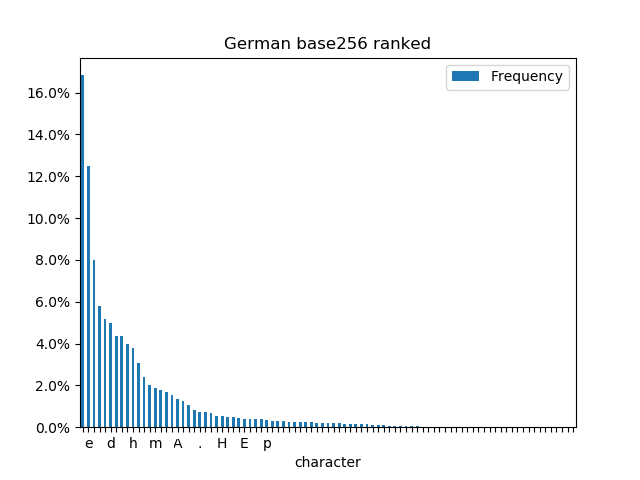
Ranking the bytes (as opposed to letters) by occurrence shows some differences and similarities.
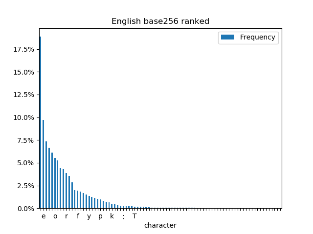
- Spaces are the most common byte in each text, but more common in English.
- The most common letter in both languages is e.
- The German chart has a “fat tail” in the low frequency bars because it uses a lot more capital letters than English.
- The letter n appears 331578 times in German but only 222748 times in English, perhaps because of strong verbs and noun plurals in German.
- The letter a appears 258985 in English, but only 180590 in German, this is probably explained by indefinite articles.
This can also be seen in a cumulative frequency diagram, in numeric order, showing jumps at the right places. The first difference is at the space character to the far left, and the difference with convergence to the right is because of umlauts and β in German.
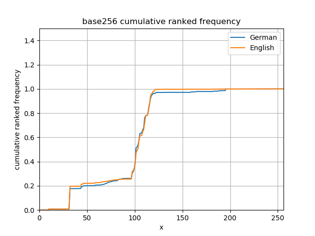
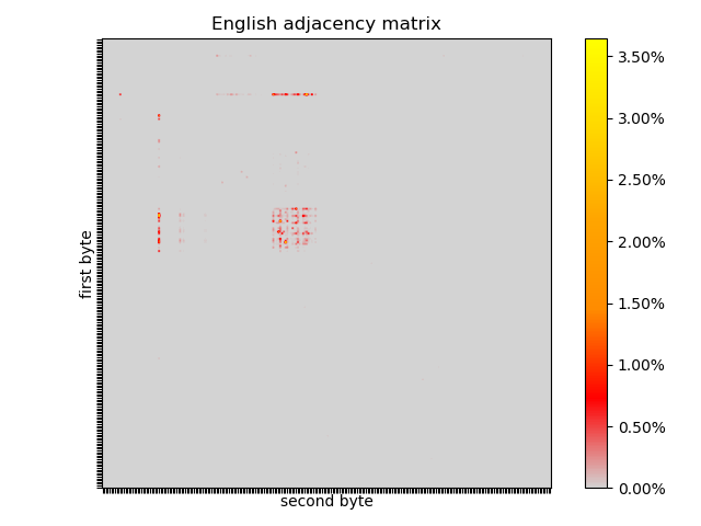
This puts the “search for the first byte” heuristic on shaky ground; some bytes are very common. Looking at frequencies of pairs of bytes and plotting them as an adjacency matrix might lead to a better heuristic, but shows some interesting patterns and is the first step to having a better data generator for benchmarking.
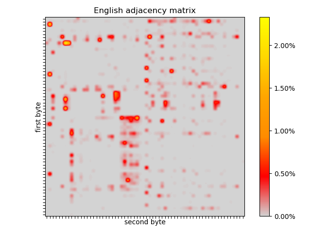
The English adjacency matrix shows how sparse the pairs of subsequent bytes are. All of the pairs are in the top left quadrant. The box where most of the combinations appear are the lower case letters. The horizontal line towards the top represents the occurences of spaces before letters, fainter in the capital letters. The vertical line towards the left is the spaces after a letter, virtually never after a capital letter, except a spot after D, an artifact of the King James Bible containing many instances of “LORD”. The rest is punctuation and book/chapter/verse markers.
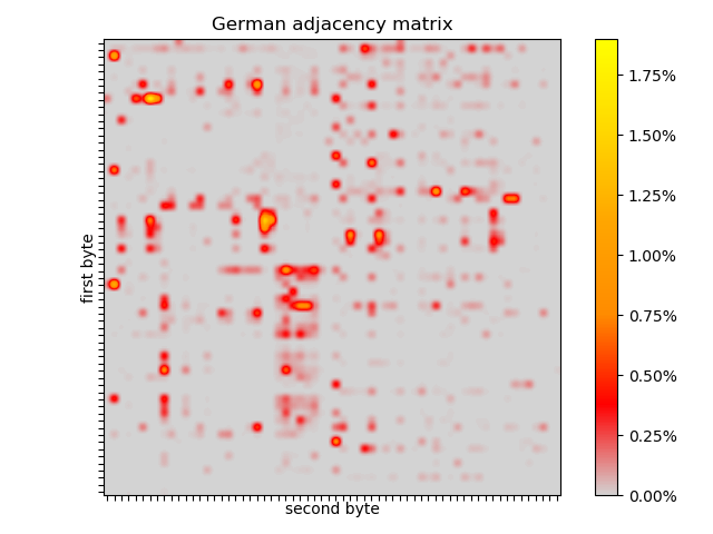
There are similarities and differences in the German adjacency matrix. There are dots outside the top left quadrant: umlauts and UTF-8 characters. The 26x26 box is there, but seems to have different hotspots. The horizontal line is there, but there is evidence of capitalised nouns after spaces. The hotspot in the vertical line is gone, but there might be a less pronounced spot after R (from “HERR”).
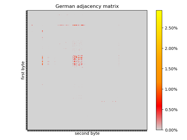
In each text, no pair occurs more than ~3% of the time, so finding the first instance of the first pair of the search term might be fruitful.
Markov chain generated English and German
Whilst it’s fun (in a way) to plot pretty pictures, the motivation for collecting histograms from texts in different languages was to benchmark frequency histogram driven linear search algorithms. I wanted a reasonable data generator with similar properties to natural languages (but this approach would also work with synthetic languages) and didn’t trust myself to think carefully enough about what properties this generator should have. Collecting the frequency histogram adjacency matrix allows its use in a very simple data generator which for each byte samples the next byte from the language’s distribution conditioned on the current byte. That is, each row in the plots above is turned into a cumulative distribution function, and for each byte, a random number uniformly distributed between zero and one is selected, and the byte corresponding to the closest entry in the CDF is selected. Next time, the selected byte is used to choose the conditional distribution to sample the next byte from.
public class MarkovChainDataGenerator implements DataGenerator {

    private final Distribution[] conditionals;
    private byte next;

    public MarkovChainDataGenerator(byte first, Distribution[] conditionals) {
        this.conditionals = conditionals;
        this.next = first;
    }

    @Override
    public byte nextByte() {
        byte current = next;
        var conditional = conditionals[next & 0xFF];
        next = conditional.nextByte();
        return current;
    }

    private static class Distribution {

        private final SplittableRandom random;

        private final byte[] bytes;
        private final double[] cdf;

        private Distribution(SplittableRandom random, byte[] bytes, double[] cdf) {
            this.random = random;
            this.bytes = bytes;
            this.cdf = cdf;
        }

        public byte nextByte() {
            double r = random.nextDouble();
            int index = Arrays.binarySearch(cdf, r);
            return bytes[index >= 0 ? index : Math.min(bytes.length, -index - 1)];
        }
    }
}
This is such a simple way to generate realistic (ish) text: all you need to do is collect the histogram and build the conditional distributions. This sometimes generates short English and German words, and reading the output is bordering on creepily reminiscent of the real languages, but reads like line noise. To get more accurate results, the process needs more memory, each byte drawn from an empirical distribution conditioned on the last $n$ bytes.
Aside from all the noise, the generator found an English word I am sure is not in the King James Bible:
“Band; asthels shit Sofanthed d t od stouthe he san, methay, spthesad y wito bopran l: adard anol, awalle, p y spe t, nd, y tich un, ne canss, maryemabe say I he oupth he we mathevidanga asey pleyed 30.”
Some of the words below are real German words, but it doesn’t really matter. All that matters for these purposes is that the letters belong next to each other, and occur with the right frequency to be German.
“10. Erend vos Daten geht, Vobich derin N s, zuschtemil, Elor te zunjararstehe rdisoph-N selssachoaun ERN zese enetetzun! undungach. vo mad und dein zoht de in s uderh s ien”
Still, this is much better than uniformly random data, easier to use programmatically than actual text, and easier to provide (seeded) variety if you are concerned about things like branch prediction.
Benchmarking First Byte Heuristic on Markovian English and German
I repeated the benchmarks with pluggable English-like and German-like data generators. With random data, finding the first byte and transitioning into a more expensive, exact match was the clear winner, because the transition doesn’t happen very often. Here’s what happened where the data length is 2000 bytes.
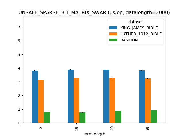
Oops. The heuristic doesn’t work well on this data. The problem is that the first byte just isn’t all that selective in either of these languages.
Serbian, Russian, Chinese (Traditional)
There are lots of other languages with their own peculiarities, both linguistic and in encoding, and they have their own distinctive signatures. I downloaded bible translations in:
- Serbian because it uses most of the same characters as English and German, has a phonetic spelling system, requiring diacritics and digraphs, and is not linguistically closely related to either.
- Russian because it uses an entirely different alphabet and character encoding, but is a Slavic language distantly related to Serbian.
- Chinese because it is different in every sense to Indo-European languages.
Whilst I can read and reason about English and German, I can’t read any of the other texts, and don’t know if they are significantly different in content; I just want to see how different the adjacency matrices are. I haven’t opened the downloaded files except with the histogram collection script, let alone attempted to make sense of them.
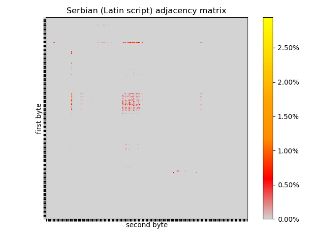
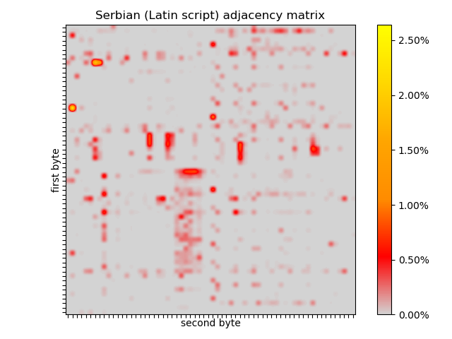
Serbian is written in two scripts: Serbian Cyrillic and Gaj’s Latin alphabet, but I used the Latin script because it was available. Serbian spelling was overhauled in the early 19th century and is entirely phonetic: one sound, one letter; one letter, one sound. This means there are no compound sounds like ch/tch in English and German, using an accent instead (č). The latin script uses several digraphs, or letters which look like two letters, such as dž, but which are represented as a single code point, typically requiring two bytes. Notably, q, w, x, and y are not in the alphabet. The encoding used is typically UTF-8 or Latin-2.
A lot of this can be seen in the adjacency matrix of the 1845 bible translation. In common with other Latin text, there is a “waffle” in the top left quadrant, stark lines corresponding to spaces, several hotspots in the bottom right quadrant, some missing letters.
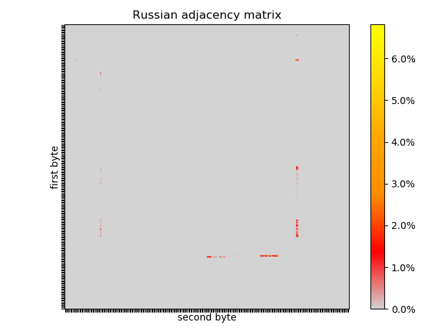
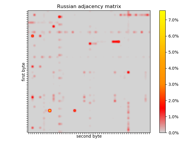
Russian is distantly related to Serbian, with some cognates and comparable grammar, but is exclusively written in Cyrillic script. The detectable difference is in encoding, UTF-8 with most code points above 256, and in the adjacency matrix flip-flopping between high and low bytes can be seen, which probably means that the generator would not produce many Russian words. Despite the linguistic relation between Serbian and Russian, the Serbian adjacency matrix is much more similar to non-Slavic English and German. That is, the first order effects are due to encoding, rather than linguistics or writing style.
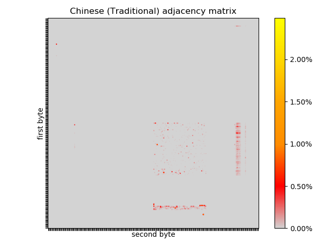
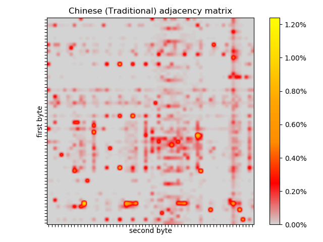
All of the languages I have considered so far are syllabalic, creating meaning by concatenating strings of letters, but Chinese doesn’t even have an alphabet. It has thousands of pictograms, which I don’t know anything about. There is very clear structure in the adjacency matrix I generated from a Chinese translation of the bible, which is different to any of the other languages considered.
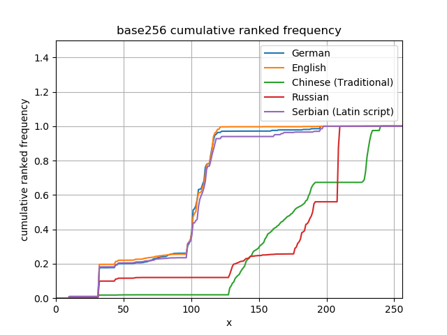
Looking at the cumulative frequencies it is obvious how different byte arrays in each of these languages will look.
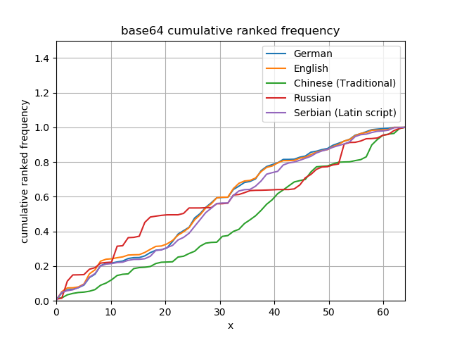
All languages look the same in Base 64
Base 64 encoding can encode any byte in a textual format using an alphabet of 64 characters. The really interesting thing about base 64 encoding comes from its mapping of each 6 bits to a single symbol of the output:
    int i = 0;
    int j = 0;
    // 3 bytes in, 4 bytes out
    for (; j + 3 < out.length && i + 2 < in.length; i += 3, j += 4) {
      // map 3 bytes into the lower 24 bits of an integer
      int word = (in[i + 0] & 0xFF) << 16 | (in[i + 1] & 0xFF) << 8 | (in[i + 2] & 0xFF);
      // for each 6-bit subword, find the appropriate character in the lookup table
      out[j + 0] = ENCODING[(word >>> 18) & 0x3F];
      out[j + 1] = ENCODING[(word >>> 12) & 0x3F];
      out[j + 2] = ENCODING[(word >>> 6) & 0x3F];
      out[j + 3] = ENCODING[word & 0x3F];
    }
The mapping crosses byte boundaries, which has the effect of shuffling or scrambling the input data onto the base 64 alphabet. This can have weird effects on compression algorithms, both beneficial and detrimental, because it changes the frequency statistics of the data. I couldn’t resist including base 64 adjacency matrices, but don’t think the improved uniformity could be capitalised on simply because mapping the search term into base 64 can’t be done independently of its offset in the containing text.
Substring search
Bit-slicing
BitMatrixSearcher requires 2KB per instance because of the structure of its masks, and SparseBitMatrixSearcher saves 1.25KB in the worst case.
This spatial overhead can be reduced to about 256 bytes by employing bit slicing, again, at a computational cost.
The basic idea is to split each byte into a high and a low nibble, and use these nibbles to look up a mask in a 16 element array of masks.
This should roughly double the number of instructions, but means only 32 masks are required in BitSlicedSearcher.
public class BitSlicedSearcher implements Searcher {

    private final long[] low;
    private final long[] high;
    private final long success;

    public BitSlicedSearcher(byte[] term) {
        if (term.length > 64) {
            throw new IllegalArgumentException("Too many bytes");
        }
        this.low = new long[16];
        this.high = new long[16];
        long word = 1L;
        for (byte b : term) {
            low[b & 0xF] |= word;
            high[(b >>> 4) & 0xF] |= word;
            word <<= 1;
        }
        this.success = 1L << (term.length - 1);
    }

    @Override
    public int find(byte[] text) {
        long current = 0L;
        for (int i = 0; i < text.length; ++i) {
            long highMask = high[(text[i] >>> 4) & 0xF];
            long lowMask = low[text[i] & 0xF];
            current = ((current << 1) | 1) & highMask & lowMask;
            if ((current & success) == success) {
                return i - Long.numberOfTrailingZeros(success);
            }
        }
        return -1;
    }
}
This is slower, but guarded by a decently selective heuristic for deciding when to enter the bit-sliced search, eliminates most spatial requirement.
BitSlicedSearcher@63021689d object externals:
          ADDRESS       SIZE TYPE                                                 PATH                           VALUE
        716eb7e28         32 BitSlicedSearcher                                                                   (object)
        716eb7e48         88 (something else)                                     (somewhere else)               (something else)
        716eb7ea0        144 [J                                                   .low                           [512, 0, 0, 193, 0, 0, 0, 0, 0, 1024, 0, 0, 4, 0, 16, 298]
        716eb7f30        144 [J                                                   .high                          [0, 0, 0, 0, 0, 0, 447, 1600, 0, 0, 0, 0, 0, 0, 0, 0]
Finding the first pair using SWAR
In several languages, the frequency of pairs of bytes is observed to be low, much lower than of common bytes.
Of course, this will likely break down for Russian, but a reasonably efficient way of finding pairs of bytes could be selective enough to wrap BitSlicedSearcher.
The branch free SWAR trick for finding the position of a byte can be adapted to pairs by increasing the distance between the holes in the mask (i.e. 0x7F7F -> 0x7FFF), but the pair may be on any alignment, so the trick is to read the data again at an offset of one byte.
public class UnsafeSWARPairFilterBitSlicedShiftAndSearcher implements Searcher, AutoCloseable {

    private final long address;
    private final long success;
    private final long pattern;


    public UnsafeSWARPairFilterBitSlicedShiftAndSearcher(byte[] term) {
        if (term.length > 64) {
            throw new IllegalArgumentException("Too many bytes");
        }
        this.address = UNSAFE.allocateMemory(16 * Long.BYTES * 2);
        UNSAFE.setMemory(address, 16 * Long.BYTES * 2, (byte) 0);
        long word = 1L;
        for (byte b : term) {
            UNSAFE.putLong(lowAddress(b & 0xF), word | UNSAFE.getLong(lowAddress(b & 0xF)));
            UNSAFE.putLong(highAddress((b >>> 4) & 0xF), word | UNSAFE.getLong(highAddress((b >>> 4) & 0xF)));
            word <<= 1;
        }
        this.success = 1L << (term.length - 1);
        this.pattern = Utils.compilePattern(term[0], term[Math.min(1, term.length - 1)]);
    }


    @Override
    public int find(byte[] text) {
        long current = 0;
        int i = 0;
        while (i + 8 < text.length) {
            long even = UNSAFE.getLong(text, BYTE_ARRAY_OFFSET + i) ^ pattern;
            long odd = UNSAFE.getLong(text, BYTE_ARRAY_OFFSET + i + 1) ^ pattern;
            long tmp0 = (even & 0x7FFF7FFF7FFF7FFFL) + 0x7FFF7FFF7FFF7FFFL;
            tmp0 = ~(tmp0 | even | 0x7FFF7FFF7FFF7FFFL);
            long tmp1 = (odd & 0x7FFF7FFF7FFF7FFFL) + 0x7FFF7FFF7FFF7FFFL;
            tmp1 = ~(tmp1 | odd | 0x7FFF7FFF7FFF7FFFL);
            int j = (Long.numberOfTrailingZeros(tmp0 | tmp1) >>> 3) & ~1;
            if (j != Long.BYTES) {
                i += j;
                for (; i < text.length; ++i) {
                    long highMask = UNSAFE.getLong(highAddress((text[i] >>> 4) & 0xF));
                    long lowMask = UNSAFE.getLong(lowAddress(text[i] & 0xF));
                    current = (((current << 1) | 1) & highMask & lowMask);
                    if (current == 0 && (i & 7) == 0 && i >= i + Long.BYTES) {
                        break;
                    }
                    if ((current & success) == success) {
                        return i - Long.numberOfTrailingZeros(success);
                    }
                }
            } else {
                i += Long.BYTES;
            }
        }
        for (; i < text.length; ++i) {
            long highMask = UNSAFE.getLong(highAddress((text[i] >>> 4) & 0xF));
            long lowMask = UNSAFE.getLong(lowAddress(text[i] & 0xF));
            current = ((current << 1) | 1) & highMask & lowMask;
            if ((current & success) == success) {
                return i - Long.numberOfTrailingZeros(success);
            }
        }
        return -1;
    }

    private long lowAddress(int position) {
        return address + Long.BYTES * position;
    }

    private long highAddress(int position) {
        return address + Long.BYTES * (position + 16);
    }

    @Override
    public void close() {
        UNSAFE.freeMemory(address);
    }
}
What is usually a more selective heuristic results in much better performance on the more structured data.
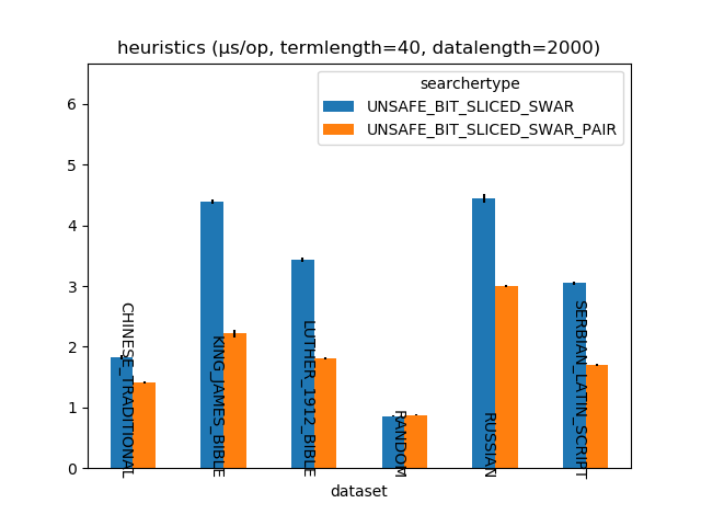
In any case ~2μs for a 2000 byte array is ~1ns/byte, at a base processor frequency of 2.6GHz with turbo-boost disabled, that’s 2.6 cycles per byte, which isn’t very fast. Given the tension between cost and selectivity of a heuristic I expect that vectorisation is necessary to get under one cycle/byte.