Sampling Whisky
Last weekend I read a post by Daniel Lemire about sampling efficiently from groups. The post presents a made up problem of sampling a student from a set of classrooms of different sizes, such that you have to pick the classroom the student should come from rather than the student. The sample needs to be unbiased, so you can’t just choose the classroom at random since they have different sizes, and each subsequent sample should be conditioned on the samples taken before. I did download the paper linked at the end of the post, but haven’t read enough of it to convince myself it is on the same topic as the post. I suspect that if I were to read it carefully, I would reach the conclusion that debating sampling algorithm efficiency is beside the point.
I thought of another practical solution to this problem, but never really liked lecture halls or classrooms very much so decided to change the setting before presenting it. Consider a whisky distillery and the chemical composition of its stock of whisky. Whisky varies wildly in flavour according to soil, malting process, whether the malt is smoked or not, the source of water. All of these factors ultimately determine its chemical composition, which gives each whisky an identifying chemical signature. After distillation, whisky sits in barrels (of various sizes) for years, developing flavour, pulling compounds out of the wood in the barrels. The age and provenance of a whisky is reflected in its taste but also in its chemical signature: whiskies of different origin and age can be distinguished by mass spectrometry. Suppose for the purposes of counterfeit detection, you need to publish a sample chemical signature of a batch of whisky before you start bottling it. Every barrel is slightly different, so you need to sample from many barrels, but anything you do sample detracts from profits because you can’t bottle it, so you want to sample as little as possible. The sample needs to be a good approximation of the signature you would obtain from all the whisky, so barrels should be sampled from with probability proportional to their size, potentially more than once. I think this silly problem is essentially the same as Daniel’s, except that the total sample size would be known ahead of time in my case.
Daniel’s approach uses a histogram which needs to be updated on each sample to get the right selection probabilities after sampling, and focuses on making updates to the histogram efficient. However, histogram updates can be avoided entirely if you can decide how many samples to take ahead of time. The alternative solution to Daniel’s is very simple: divide the total amount of whisky by the size of each sample, and imagine the whisky were stored conveniently in “addressable units” of this size, laid out in an order determined by the barrels the units belong to. Then, rather than choose the barrel, you choose the unit of whisky to sample, and figure out which barrel it belongs to from its position. The only challenge is generating unit positions which are unbiased to any barrel or set of barrels.
Given that you know how many addressable units of whisky you have, $N$, you can choose random numbers from $[0,N)$, and store these in a set to reject collisions, but this requires $\mathcal{O}(k)$ space, where $k$ is the sample size. Generating positions sequentially avoids spatial overhead, and it’s just a question of which distribution to generate from.
Firstly, if you generate positions sequentially, when you have already taken $n$ samples of $k$, you must not select a position $i > N - k + n$, because if you do you won’t get a complete sample without going backwards. If you go backwards, you need to remember which values you have already sampled, which entails spatial overhead. You also need the numbers to spread out uniformly in $[0,N)$, so choosing a number from $U(i, N-k+n)$ probably won’t cut it because it leads to clumping towards the end.
Imagine scanning over the addressable units and choosing which to accept for the sample. Each should be accepted with probability $\frac{k-n}{N-i}$, that is, you accept in proportion to how many you need to take from what’s left. This is equivalent to selecting the next position $i$ with probability $\mathbb{P}(i=j) = \frac{k-n}{N-j}$ (this is the probability distribution of the intervals between each successful trial). Jeffrey Vitters presented several algorithms for generating these indices in the 1980s in Faster Methods for Random Sampling.
I read this paper earlier this year and fleshed out the derivations of the probability density function of the gaps between each sample.
This probability density function can be approximated by drawing a value from a geometric distribution with parameter $\frac{k-n}{N-i}$ for each sampled value. This is an $\mathcal{O}(k)$ algorithm, produces samples in sorted order, and doesn’t need to make expensive (logarithmic or linear) updates to a histogram. The only drawback is that you must choose $k$ ahead of time, whereas Daniel’s algorithm allows you to keep sampling for as long as you like.
I implemented this, with an extra step to infer the barrel the unit belongs to, in Java:
public class GeometricDistributionSampler implements BucketSampler {

  @Override
  public int sample(int[] histogram, int[] sample) {
    int[] cumulativeHistogram = Arrays.copyOf(histogram, histogram.length);
    for (int i = 1; i < cumulativeHistogram.length; ++i) {
      cumulativeHistogram[i] += cumulativeHistogram[i-1];
    }
    double remainingToSample = sample.length;
    double remainingToSampleFrom = cumulativeHistogram[cumulativeHistogram.length - 1];
    int pos = 0;
    int bucket = 0;
    double p = remainingToSample/remainingToSampleFrom;
    int nextItem = (int)(log(ThreadLocalRandom.current().nextDouble())/log(1-p)) + 1;
    while (pos < sample.length) {
      while (bucket < cumulativeHistogram.length
              && nextItem >= cumulativeHistogram[bucket]) {
        ++bucket;
      }
      sample[pos++] = bucket;
      int gap = (int)(log(ThreadLocalRandom.current().nextDouble())/log(1-p)) + 1;
      nextItem += gap;
      remainingToSampleFrom -= gap;
      --remainingToSample;
      p = remainingToSample/remainingToSampleFrom;
    }
    return pos;
  }
}
Out of curiosity, I compared this with Daniel’s algorithm (his code, but refactored to produce a sample of a predefined size):
public class LemireSmarter implements BucketSampler {
  @Override
  public int sample(int[] histo, int[] sample) {
    int sum = 0;
    for (int i : histo) {
      sum += i;
    }
    // build tree
    int l = 0;
    while ((1 << l) < histo.length) {
      l++;
    }
    int[] runninghisto = Arrays.copyOf(histo, histo.length);
    int level = 0;
    for (;
         (1 << level) < runninghisto.length; level++) {
      for (int z = (1 << level) - 1; z + (1 << level) < runninghisto.length; z += 2 * (1 << level)) {
        runninghisto[z + (1 << level)] += runninghisto[z];
      }
    }
    int maxlevel = level;
    int pos = 0;
    while (pos < sample.length) {
      int y = ThreadLocalRandom.current().nextInt(sum); // random integer in [0,sum)
      // select logarithmic time
      level = maxlevel;
      int position = (1 << level) - 1;
      int runningsum = 0;
      for (; level >= 0; level -= 1) {
        if (y > runningsum + runninghisto[position]) {
          runningsum += runninghisto[position];
          position += (1 << level) / 2;
        } else if (y == runningsum + runninghisto[position]) {
          runninghisto[position] -= 1;
          break;
        } else {
          runninghisto[position] -= 1;
          position -= (1 << level) / 2;
        }
      }
      sample[pos++] = position;
      sum -= 1;
    }
    return pos;
  }
}
I was pleased to see that Vitters’ approach from the early 80s did fairly well (lower is better)!
| Benchmark | Mode | Threads | Samples | Score | Score Error (99.9%) | Unit | Param: k | Param: p |
|---|---|---|---|---|---|---|---|---|
| geometric | avgt | 1 | 5 | 36.247117 | 0.066174 | us/op | 500 | 4096 |
| geometric | avgt | 1 | 5 | 42.097286 | 0.064073 | us/op | 500 | 8192 |
| geometric | avgt | 1 | 5 | 67.283053 | 5.425246 | us/op | 1000 | 4096 |
| geometric | avgt | 1 | 5 | 72.118459 | 6.762172 | us/op | 1000 | 8192 |
| geometric | avgt | 1 | 5 | 129.392192 | 1.111991 | us/op | 2000 | 4096 |
| geometric | avgt | 1 | 5 | 131.812448 | 1.028063 | us/op | 2000 | 8192 |
| lemireSmarter | avgt | 1 | 5 | 71.844391 | 9.460850 | us/op | 500 | 4096 |
| lemireSmarter | avgt | 1 | 5 | 88.622040 | 9.059404 | us/op | 500 | 8192 |
| lemireSmarter | avgt | 1 | 5 | 133.558966 | 13.322686 | us/op | 1000 | 4096 |
| lemireSmarter | avgt | 1 | 5 | 163.835369 | 1.703278 | us/op | 1000 | 8192 |
| lemireSmarter | avgt | 1 | 5 | 274.023876 | 1.230904 | us/op | 2000 | 4096 |
| lemireSmarter | avgt | 1 | 5 | 307.959800 | 1.938573 | us/op | 2000 | 8192 |
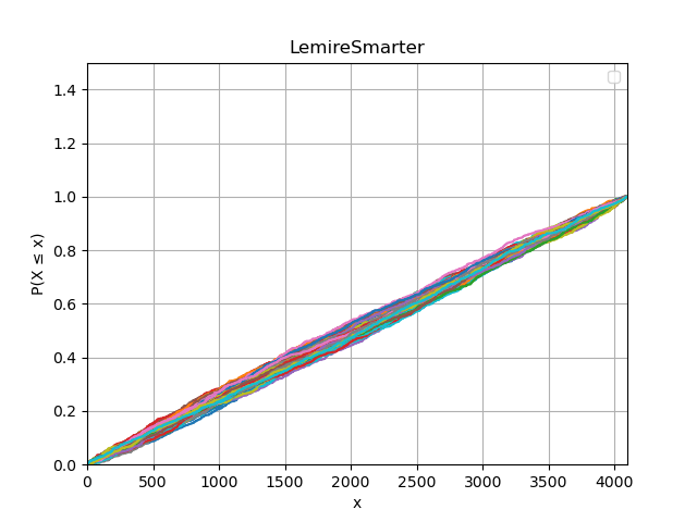
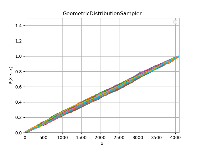
Since I am probably long past my mathematical prime, I wanted to check how uniform the samples from each algorithm were, so generated samples of 500 from 4096 barrels for each algorithm 100 times, and plotted the cumulative density. Getting straight lines means the sample is more or less uniform (i.e. not biased to any of the barrels), and it looks like the algorithms both generate similar output. So, this is an apples to apples comparison, albeit not exploiting the full capabilities of Daniel’s algorithm